FuncFit when some data in asymptotic/imaginary domain after fitting


Hello,
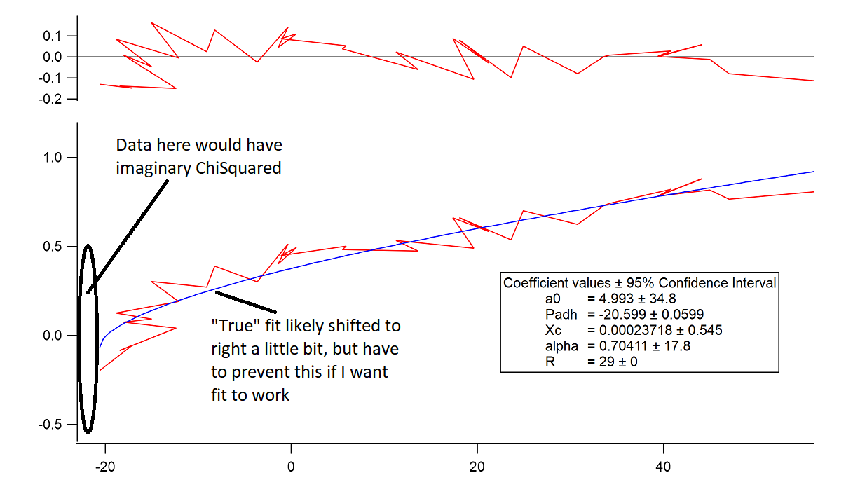
I am trying to fit some data in the vicinity of where a user function, which has a sqrt(1-x)-like term, becomes imaginary i.e. where X>1. The true functional dependence likely passes through the center of the data spread, but in that case ChiSquared for some of the data points will be imaginary since the fit function at those X-values will be imaginary.
I mention this upfront, because I suspect (but don't know that) this effect is responsible for poor convergence of the fit if I leave it totally unconstrained. I know the fit is poor because it converges with coefficients close to whatever I enter as coefficient initial guesses, even if the guesses are very poor.
I tried increasing the max iterations for cases where the fit hits the 40iteration limit, which doesn't help the fit and there is always "convergence" (to a bad fit) before 100 iterations in any case.
I tried lowering the V_FitTol to the minimum allowed, which doesn't help the fit.
I tuned on and looked at M_Iterates, which didn't tell me much, aside from showing that the fit will try a coefficient early on that will force a lot of the data to have imaginary ChiSquared, then stays in the vicinity of the initial guess thereafter. The small variation in coefficient guesses in later iterations appears to allow the bad ChiSquare value to stabilize enough to meet the convergence criterion, even though the magnitude of ChiSquared is high.
I tried calculating the correlation matrix, and all of the off-diagonal elements are far enough from 1 (<0.9) that I don't think I have an identifiability problem with the user function coefficients.
The one thing that does work is to constrain the coefficients so the ChiSquare of every data point cannot become imaginary. In that case, I can feed bad guesses to the fit and it will always converge quickly (<10iterations) to basically the same fit that looks good. This is a workable solution, but the fit always converges to run through the data point on the domain that leads to imaginary ChiSquared datapoints i.e. it converges to edge of the constraint I enter. To me, this suggests that the "actual" best fit would run through the middle of the envelope of these datapoints. I attach an image showing this best fit and also where I think the real best fit actually is. I also attach a minimal experiment file with this data and fitting function.
Is there a non-onerous way to deal with this problem, or should I just live with my workaround and whatever (relatively small) error it introduces? I wanted to check, because it would be better not to have to have this error source if it can be avoided. Am I diagnosing the problem correctly? I think the imaginary ChiSquared values are the problem, but I don't really have clear proof of it and I don't have other ideas about how to look more deeply into the details of the fit trajectory.
This seems like a problem that would be generic to all scientific software doing least-squares fitting, but I couldn't find similar discussions with a google search.
Thank you for any ideas or recommendations you share.
I think the only way to handle that is to make your fitting function return a real value for X < Padh (I think I have that right, eh?). I tried adding this to your fitting function:
That makes the function symmetric about Padh. But when I ran your fitting function, it resulted in a major distortion of the entire fit curve. So it is not at all clear how to patch up your fitting function appropriately.
What you really need is a function that magically returns the "expected" Y value for the "fixed up" X value. I don't know how to do that.
I also note that it looks like you have noise in the X direction, and that is really the crux of the issue. You may also need to use ODR fitting: DisplayHelpTopic "Errors in Variables: Orthogonal Distance Regression". But that will still require solving the issue of an appropriate way to make the fit function return real values.
Sudden thought- is there any possibility of fitting X vs Y to the inverse of your function? Possibly finding the inverse is not possible...
January 9, 2023 at 10:58 am - Permalink
Thank you. You're right, there is some experimental noise in X so I get some data where the physics of the situation says there should not be any. Your response alerted me to the fact that you can fit piecewise functions, which I was unaware of but now see there is an entire section of the manual about. Instead of making the function symmetric, I tried setting it to Xc for P<Padh, so ChiSquared is large for datapoints outside the function's domain of validity but not gigantic:
After constraining the output to reasonable values, this does seem to result in a reasonable fit, although the output still seems to have Padh migrate to the position of the smallest P in the dataset. I assume this is because for this particular dataset (I have other curves with many more points) those few somewhat large ChiSquared values result in Padh getting pushed downward to reduce their ChiSquared contribution:
M_iterates (attached) does seem to show the alpha value getting stuck at 1 after trying some disallowed negative values at early iterations. With Padh constrained like I had it before, output alpha was ~0.85 resulting in slightly better final ChiSquared of V_chisq= 0.253, vs 0.266 for the current fit, which is why I think alpha got stuck.
January 9, 2023 at 12:14 pm - Permalink
For anyone who runs into a similar problem with fitting piecewise functions, it turns out I needed adjust the epsilon values upward from their defaults. As usual, once I found the solution I discovered that there is a whole section of the manual that talks about this, and even warns that the default epsilons may not work adequately for piecewise functions.
January 13, 2023 at 09:11 am - Permalink
Ah, I hadn't thought of adjusting the epsilon for this.
January 13, 2023 at 09:53 am - Permalink
But you did write the response to someone asking a different question about bad fits which suggested adjusting epsilon to him/her (and now me).
January 13, 2023 at 09:55 am - Permalink
Yes. That was probably more than five minutes ago :) I'm getting old, and my memory was never very good!
January 13, 2023 at 02:25 pm - Permalink
I am going to ask from a first principles consideration. This appears to be analysis from so-called force-distance curves in atomic force microscopy. You are fitting to the potential well function that is mapped by the displacement of the tip as a function of tip's distance from a surface. You are fitting entirely to the repulsion portion of the curve.
If I have this correct, then let me reconsider your analysis from first principles to try to fix the problems you are having during curving fitting.
First, for true potential versus distance curves, the zero point the position axis should be at the hard well repulsion point plus a typically unknown offset value, where the offset value typically accounts for the radius of the atoms that first contact each other at the hard-wall repulsion point. Forgoing the unknown value, the zero point of displacement is certainly never set at the bottom of the potential well. See the first attached picture.
The above being said, I understand however why you set the zero point at the bottom of the well. You want to remove all negative tip positions from the curve fitting because they represent the pull-off portion. OK.
Now let's tackle the negative values in tip deflection.
The best fix for this is to renormalize your tip displacement values. First, use a dimensionless potential form U/Uo, where Uo is the value at the bottom of the potential well. In this case, Uo is the value at the bottom of your tip deflection, approximately -20. The next step is to put the bottom of your potential well at zero. This simply means that you add +1 to the relative potential. The end result is that you plot Psi = (U/Uo) + 1 versus tip displacement. The second figure is the plot where I distinguish the two tracks (advancing and receding tip) by different markers.
You should now modify your fitting function to fit to the solid circles. You will not have singularities. You can back-calculate the resulting dimensionless fitting parameters to their real, absolute parameters by deconstructing the fitting equation.
January 13, 2023 at 03:43 pm - Permalink
This is almost what I am doing, but my sample is much softer and my tip much blunter than your analysis assumes. In my case, I am elastically deforming a somewhat soft sample with the tip, so the measurement is not particularly sensitive to the shape of the potential well for the undeformed state. My tip is a special one that is almost perfectly round, has a hard coating, and is atomically smooth with a known (from e- microscopy) radius of 29nm in this case. This lets me use analytic equations to model the contact mechanics. Typically you can use simple DMT or JKR contact mechanics for this sort of thing, depending on whether the sample is stiff with low adhesion or soft with high adhesion, but I have bad luck because this sample occupies an intermediate state where I have to use a somewhat more complicated intermediate model with lots of parameters from here: https://www.sciencedirect.com/science/article/pii/S0021979700968085
Not only that, based on the literature, I think I am the first person to ever try to model this intermediate state for real data where the alpha parameter doesn't disappear, so there might be some problems, like how I've started to see identifiability problems in the correlation matrix on most of my fits even after cleaning up some things like the epsilon parameter and getting the piecewise fitting function to work, suggesting even a good fit might not be unique.
The data I shared has already been compensated for the cantilever beam bending, so the positive values are displacement of the tip into the sample and on retract the sample forms a bit of a neck and stays in contact above the initial sample surface under tensile loading.
I appreciate you taking a look at my data, and you've helped me probably half a dozen times in the past.
January 13, 2023 at 04:46 pm - Permalink