You can use convolution to compute the response of a linear system to an input signal. The linear system is defined by its impulse response. The convolution of the input signal and the impulse response is the output signal response. Convolution is also the time-domain equivalent of filtering in the frequency domain.

Igor Pro® implements general convolution with the Convolve operation. (Smoothing is also a form of convolution) To use the Convolve operation, you can choose Convolve from the Analysis menu:

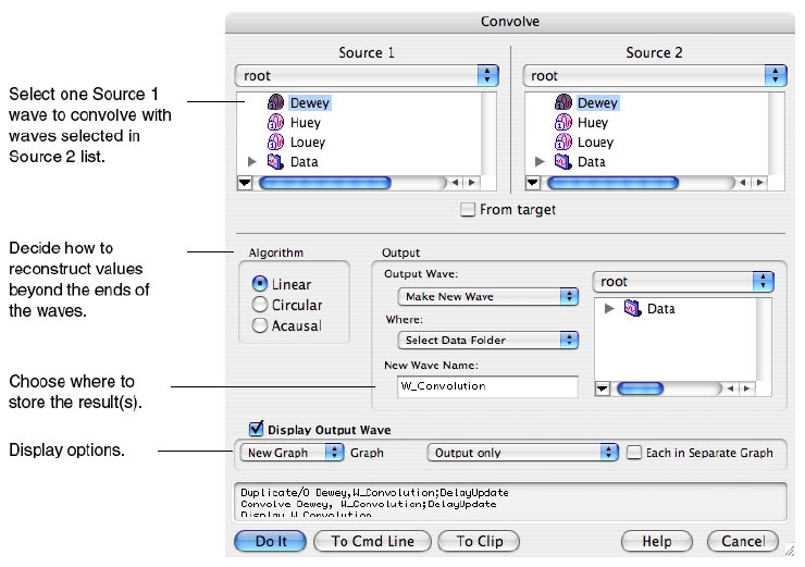
The built-in Convolve operation computes the convolution of two waves named "source" and "destination" and overwrites the destination wave with the results. The operation can also convolve a single source wave with multiple destination waves (overwriting the corresponding destination wave with the results in each case). The Convolve dialog allows for more flexibility by pre-duplicating the second waves into new destination waves.

If the source wave is real-valued, each destination wave must be real-valued and if source wave is complex, each destination wave must be complex, too. Double and single precision waves may be freely intermixed; the calculations are performed in the higher precision.

Convolve combines neighboring points before and after the point being convolved, and at the ends of the waves not enough neighboring points exist. This is a general problem in any convolution operation; the smoothing operations use the End Effect pop-up to determine what to do. The Convolve dialog presents three algorithms in the Algorithm group to deal with these missing points.

The Linear algorithm is similar to the Smooth operation´s Zero end effect method; zeros are substituted for the values of missing neighboring points.

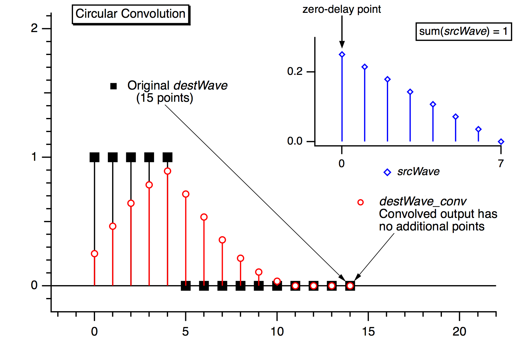
The Circular algorithm is similar to the Wrap end effect method; this algorithm is appropriate for data which is assumed to endlessly repeat.

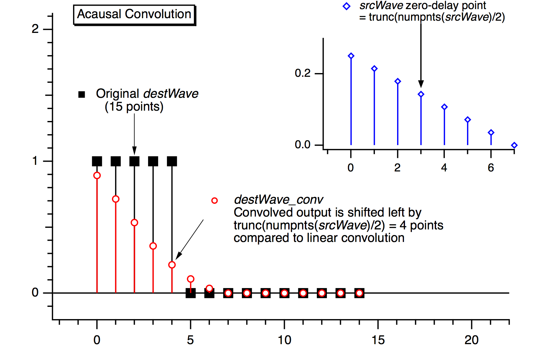
The acausal algorithm is a special case of Linear which eliminates the time delay that Linear introduces.

Depending on the algorithm chosen, the number of points in the destination waves may increase by the number of points in the source wave, less one. For linear and acausal convolution, the destination wave is first zero-padded by one less than the number of points in the source wave. This prevents the "wrap-around" effect that occurs in circular convolution. The zero-padded points are removed after acausal convolution, and retained after linear convolution.

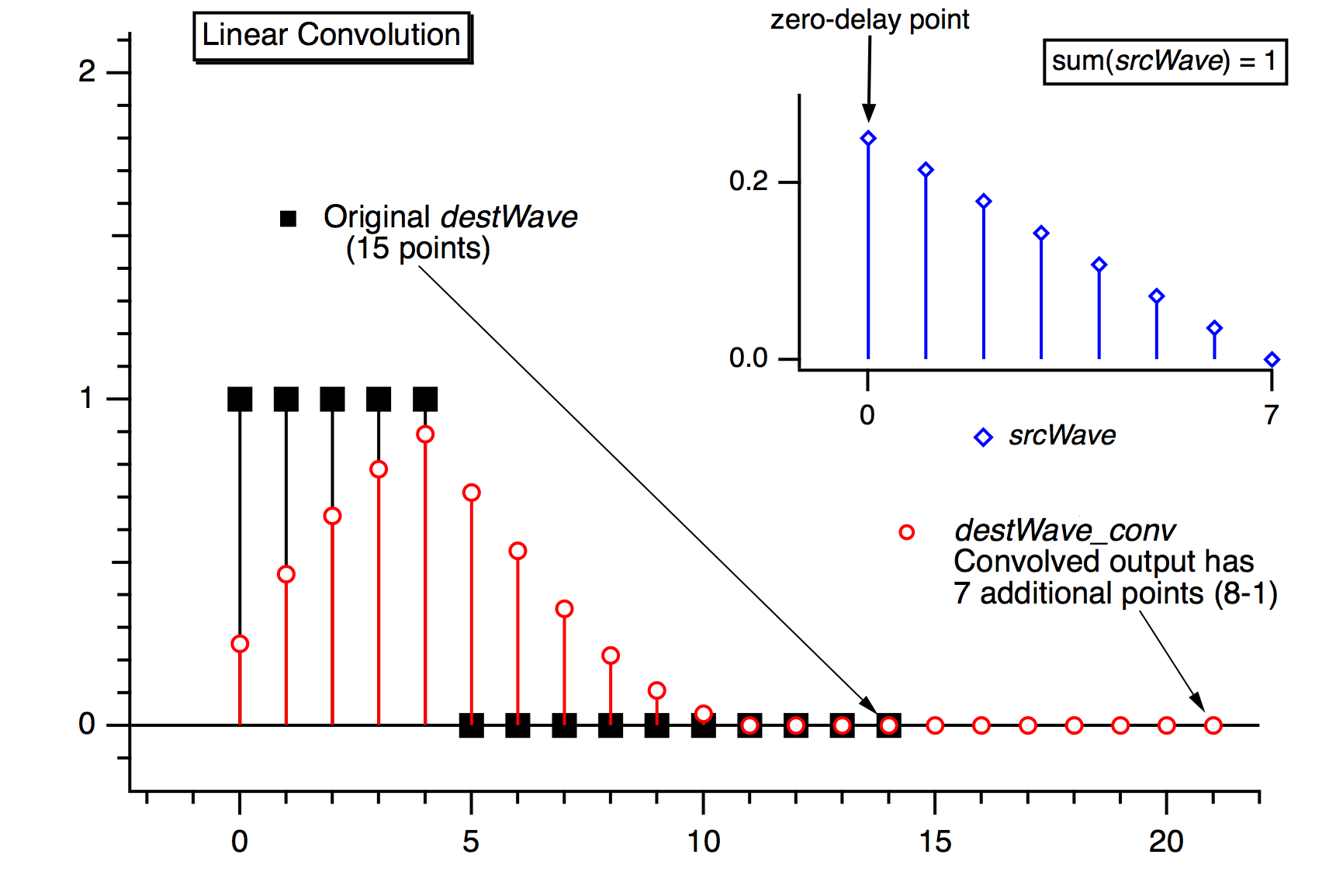
Use linear convolution when the source wave contains an impulse response (or filter coefficients) where the first point of srcWave corresponds to no delay (t = 0).

Use circular convolution for the case where the data in the source wave and the destination waves are considered to endlessly repeat (or "wrap around" from the end back to the start), which means no zero padding is needed.

Use acausal convolution when the source wave contains an impulse response where the middle point of the source wave corresponds to no delay (t = 0).

Correlation

You can use correlation to compare the similarity of two sets of data. Correlation computes a measure of similarity of two input signals as they are shifted by one another. The correlation result reaches a maximum at the time when the two signals match best. If the two signals are identical, this maximum is reached at t = 0 (no delay). If the two signals have similar shapes but one is delayed in time and possibly has noise added to it then correlation is a good method to measure that delay.

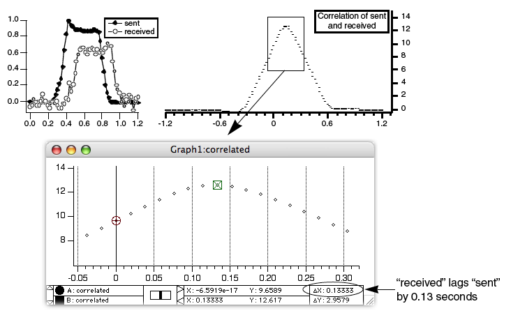
Igor implements correlation with the Correlate operation. The Correlate dialog in the Analysis menu works similarly to the Convolve dialog. The source wave may also be a destination wave, in which case afterward it will contain the "auto-correlation" of the wave. If the source and destination are different, this is called "cross-correlation".

The same considerations about combining differing types of source and destination waves applies to correlation as to convolution. Correlation must also deal with end effects, and these are dealt with by the circular and linear correlation algorithm selections.

Pearson´s r Correlation

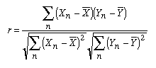
You can compute a single correlation value (called Pearson´s r) for the correlation of two data sets using Igor´s StatsLinearCorrelationTest operation. Pearson´s linear correlation coefficient r is given by:

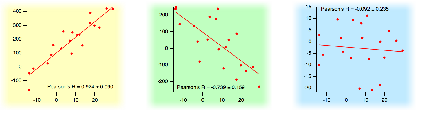
Pearson´s r reflects the degree of linear relationship between the two data sets. Its value is between -1 and +1. A value of +1 means that there is a perfect positive linear relationship between the two data sets. A value of -1 means that there is a perfect negative linear relationship, and a value of 0 means there is no linear relationship at all between the data sets. In practice the value will be some intermediate number. These three graphs show three different data sets plotted versus a common reference data set. The three data sets have differing amounts of correlation with the the reference data set. (A line fit is also shown for reference, but Pearson´s r is not an indication of the line fit´slope.)

References

• Press, William H. [et. al.], "Fourier and Spectral Applications", sec. 13, Numerical Recipes in C, 2nd ed., Cambridge University Press, 1992.
• Press, William H. [et. al.], "Linear Correlation", sec. 14.5, Numerical Recipes in C, 2nd ed., Cambridge University Press, 1992.