You can perform (linear) regression analysis using Igor's curve fitting operations.. StatsLinearRegression provides more statistical information/tests for single and multiple regressions.
1. Simple linear regression.
Start by creating a wave with a known slope and additive Gaussian noise.
Make/O/N=100 data1=x+gnoise(4)
The simple linear regression analysis is obtained by:
StatsLinearRegression /T=1/Q data1
The results appear in the Linear Regression table (shown transposed):
| N | 100 |
| a | -0.912472 |
| b | 1.01654 |
| xBar | 49.5 |
| yBar | 49.4064 |
| sumx2 | 83325 |
| sumy2 | 87529 |
| sumxy | 84703.4 |
| Syx | 3.81255 |
| F | 5923.74 |
| Fc | 3.93811 |
| r2 | 0.983726 |
| Sb | 0.0132077 |
| t | |
| tc | 1.98447 |
| L1 | 0.990332 |
| L2 | 1.04275 |
When a slope is not specified the null hypothesis is that the slope is zero and the t-statistic is not relevant. The regression results above clearly reject this hypothesis with regression line given by:
y=-0.912472+1.01654*x.
To plot the regression and the data curves execute the commands:
Duplicate/O data1,regression1
regression1=-0.912472+1.01654*x
Display/K=1 data1,regression1
ModifyGraph lsize(regression1)=2,rgb(regression1)=(0,0,0)
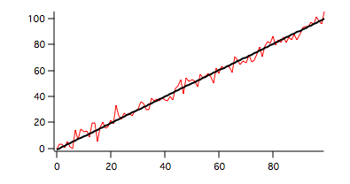
Here the red trace corresponds to our input data and the black trace is the regression line.
You can create confidence interval waves and prediction interval waves using
StatsLinearRegression /T=1/Q/BCIW/BPIW data1
You can now add the two bands to the graph:
AppendToGraph data1_CH,data1_CL,data1_PH,data1_PL
ModifyGraph rgb(data1_CH)=(0,65535,0),rgb(data1_CL)=(0,65535,0)
ModifyGraph rgb(data1_PH)=(0,0,65535),rgb(data1_PL)=(0,0,65535)
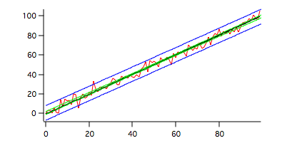
Here the green traces correspond to the confidence interval while the blue traces correspond to the prediction interval (default single prediction).
2. Zero slope hypothesis
To see the results of the zero-slope hypothesis test on different data set we generate data that have zero slope and random noise:
Make/O/N=100 data2=10+gnoise(4)
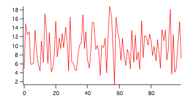
A graph pf data2 is shown above. To run the test execute the command:
StatsLinearRegression /T=1/Q data2
| N | 100 |
| a | 9.44344 |
| b | 0.00449769 |
| xBar | 49.5 |
| yBar | 9.66608 |
| sumx2 | 83325 |
| sumy2 | 1505.25 |
| sumxy | 374.77 |
| Syx | 3.91695 |
| F | 0.109865 |
| Fc | 3.93811 |
| r2 | 0.00111981 |
| Sb | 0.0135694 |
| t | |
| tc | 1.98447 |
| L1 | -0.0224303 |
| L2 | 0.0314257 |
As expected, F<Fc and the hypothesis of zero slope must be accepted.
3. Specific slope hypothesis
Testing the hypothesis that the slope b=beta0. Using the wave data1 which was generated with a unit slope we have:
StatsLinearRegression /T=1/Q/B=1.0 data1
It should be obvious from the definitions of L1 and L2 that any value of beta0 outside the range [L1,L2] will be rejected.
4. Linear regression for more than one wave.
Make/O/N=100 data3=4+x+gnoise(4)
Make/O/N=100 data4=5+x+gnoise(5)
You can run the linear regression test on multiple samples using the command:
StatsLinearRegression /T=1/Q data1,data3,data4
The results are displayed in the Linear Regression table and in the Linear Regression MC table.
Linear Regression table:
| data | data3 | data4 | ||
| N | 100 | 100 | 100 | |
| a | -0.912472 | 4.10709 | 4.37794 | |
| b | 1.01654 | 0.993232 | 0.993211 | |
| xBar | 49.5 | 49.5 | 49.5 | |
| yBar | 49.4064 | 53.272 | 53.5419 | |
| sumx2 | 83325 | 83325 | 83325 | |
| sumy2 | 87529 | 83725. | 85298.4 | |
| sumxy | 84703.4 | 8276 | 82759.3 | |
| Syx | 3.81255 | 3.94368 | 5.62508 | |
| F | 5923.74 | 5285.34 | 2597.77 | |
| Fc | 3.9381 | 3.9381 | 3.93811 | |
| r2 | 0.983726 | 0.981796 | 0.963647 | |
| Sb | 0.0132077 | 0.013662 | 0.0194868 | |
| t | ||||
| tc | 1.98447 | 1.98447 | 1.98447 | |
| L1 | 0.990332 | 0.96612 | 0.95454 | |
| L2 | 1.04275 | 1.02034 | 1.03188 |
Linear Regression MC table:
| Ac | 249975 |
| Bc | 250224 |
| Cc | 256552 |
| SSp | 6049.51 |
| SSc | 6079.72 |
| SSt | 7150.35 |
| DFp | 294 |
| DFc | 296 |
| DFt | 298 |
| Slopes F | 0.734116 |
| Slopes Fc | 3.02647 |
| CoincidentalRegression F | 13.375 |
| CoincidentalRegression Fc | 2.40235 |
| Elevations F | 26.0627 |
| Elevations Fc | 3.02626 |
In this case the slopes' test results in F<Fc so the hypothesis of equal slopes is accepted while elevation's test results F>Fc implies that the equal elevations hypothesis is rejected as is the possibility of coincidental regression.
You can also test waves of unequal lengths as in the following example:
Make/O/N=150 data5=x+gnoise(4)
Make/O/N=100 data6=x+gnoise(5)
StatsLinearRegression /T=1/Q data1,data5,data6
| Ac | 447888 |
| Bc | 449403 |
| Cc | 457496 |
| SSp | 6549.12 |
| SSc | 6571.72 |
| SSt | 6614.3 |
| DFp | 344 |
| DFc | 346 |
| DFt | 348 |
| Slopes F | 0.593541 |
| Slopes Fc | 3.02197 |
| CoincidentalRegression F | 0.855888 |
| CoincidentalRegression Fc | 2.3979 |
| Elevations F | 1.12087 |
| Elevations Fc | 3.02182 |
In this case both the slopes and the elevations are determined to be the same. The single test for coincidental regression would also indicate that the three waves have coincident regressions.
5. Dunnett's multi-comparison test for elevations.
You can perform Dunnett's multi-comparison test on the elevations of the several waves. In this example we define the first input wave as the control sample (/DET=0):
StatsLinearRegression /T=1/Q/DET=0 data1,data3,data4,data5,data6
The operation computes the linear regression and the general multi-comparison as described above. In addition it displays Dunnett's MC Elevations table for tests of each input wave against the control wave:
| Pair | SE | q | qp | Conclusion |
| 1_vs_0 | 0.641955 | 6.02176 | 2.16539 | 0 |
| 2_vs_0 | 0.641955 | 6.44208 | 2.16539 | 0 |
| 3_vs_0 | 0.615424 | 0.127039 | 2.16539 | 1 |
| 4_vs_0 | 0.641955 | 1.23037 | 2.16539 | 1 |
The table indicates that the equal elevation hypothesis is rejected for the pairs data3-data1 and data4-data1. The hypothesis is accepted for the other combinations.
6. The Tukey test for multiple regressions
The test depends on the F tests for the slopes. If the slopes are determined to be the same then the Tukey test compares elevations. Otherwise, the Tukey test performs a multi-comparison of slopes.
StatsLinearRegression /T=1/Q/TUK data1,data3,data4,data5,data6
Since the slopes were determined to be the same, the Tukey test was performed on the elevations and the results are displayed in the Tukey MC Elevations table:
| Pair | SE | q | qc | Conclusion |
| 4_vs_0 | 0.45393 | 1.7400 | 3.87073 | 1 |
| 4_vs_ | 0.45393 | 6.77604 | 3.87073 | 0 |
| 4_vs_2 | 0.45393 | 7.37047 | 3.87073 | 0 |
| 4_vs_3 | 0.43517 | 1.63536 | 3.87073 | 1 |
| 3_vs_0 | 0.43517 | 0.17966 | 3.87073 | 1 |
| 3_vs_ | 0.43517 | 8.7035 | 3.87073 | 0 |
| 3_vs_2 | 0.43517 | 9.32356 | 3.87073 | 0 |
| 2_vs_0 | 0.45393 | 9.11048 | 3.87073 | 0 |
| 2_vs_ | 0.45393 | 0.594429 | 3.87073 | 1 |
| 1_vs_0 | 0.45393 | 8.51605 | 3.87073 | 0 |
As expected input waves 1 and 2 do not match the elevations of the other waves.
7. Regression analysis with multiple Y values for each X value
When the data has multiple Y values for each X value you need to store the input as a 2D wave there each column represents one set of Y values. In this example the wave dataMYV consists of 30 rows and 6 columns so there are at most 6 Y values for each X. There are 6 NaNs representing missing values or padding used to format the input for the operation in case the number of Y-values is not the same for all x values. The X-values are implied by the wave scaling of the rows with start=1 and delta=3.
StatsLinearRegression /T=1/Q/MYVW={*,dataMYV}
The results are displayed in the "Linear Regression" table (shown transposed):
| N | |
| 174 | |
| a | -0.564705 |
| b | 2.01551 |
| xBar | 44.2586 |
| yBar | 88.639 |
| sumx2 | 117111 |
| sumy2 | 485408 |
| sumxy | 236039 |
| amongGroupsSS | 477052 |
| amongGroupsDF | 29 |
| withinGroupsSS | 8355.47 |
| withinGroupsDF | 144 |
| devLinearitySS | 1312.81 |
| devLinearityDF | 28 |
| F | 0.808045 |
| Fc | 1.55463 |
| F2 | 8463.47 |
| F2c | 3.89609 |
| r2 | 0.980082 |
| Syx | 7.4974 |
The F value is smaller than the critical Fc which implies that the regression of the data is indeed linear. The value of F2 is much greater than the critical value F2c which implies that the hypothesis of slope b=0 has to be rejected.

Forum

Support

Gallery
Igor Pro 10
Learn More
Igor XOP Toolkit
Learn More
Igor NIDAQ Tools MX
Learn More