Many image processing operations result in changes to the image's histogram. The class of histogram modifications which we consider here include operations where the changes to pixel levels are computed so as to change the histogram in a particular way.

Histogram Stretching

The simplest form of histogram modification is histogram stretching. For example, if the image is under-exposed its values would only occupy the lower part of the dynamic range. You can perform the histogram stretching for an 8-bit image using:

The normalization variable makes the subsequent operation a bit more efficient.

The following images illustrate histogram stretching. In each case the image is shown on the left and the corresponding luminance histogram is shown on the right. Below the image we show the histograms of the RGB components.

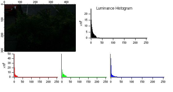
An example of a dark image (short exposure) together with its luminance and RGB histograms.

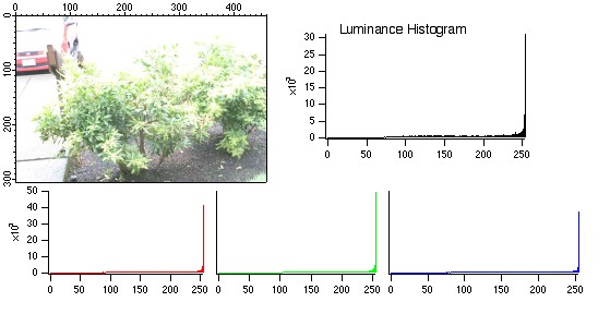
An example of an over-exposed image together with its luminance and RGB histograms. There is usually not much that one can do to improve such an image as many pixels are saturated.

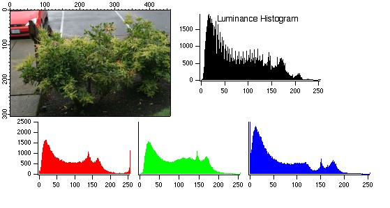
An example of an standard image together with its luminance and RGB histograms.

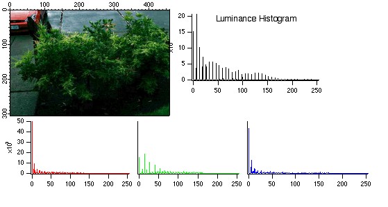
A stretched histogram image that was obtained from the dark image (top) and mapped with a high normalization factor. The stretching of the histogram was actually performed on the luminance channel after converting the original image to HSL color space. Note that the bin distribution of the different histograms are not contiguous (cf. the continuous histograms of the normally exposed image above). This can sometimes be used to identify images whose histogram has been stretched.

Histogram Equalization

Histogram equalization is a method for "spreading" the histogram of pixel levels more evenly.

In more complicated cases, the global histogram may not be a good representation for local statistics in two parts of the image. In such cases it is best to use an adaptive histogram equalization where you can divide the image into several rectangular domains, compute an equalizing histogram and modify levels so that they match across boundaries. Depending on the nature of the non-uniformity of the image, you might consider using Background Removal

The following images illustrate the differences between global and adaptive histogram equalization.

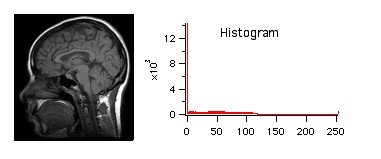
A figure showing the standard MRI image with the corresponding gray-scale histogram. The histogram has a peak at minimum intensity consistent with the relatively dark nature of the image.

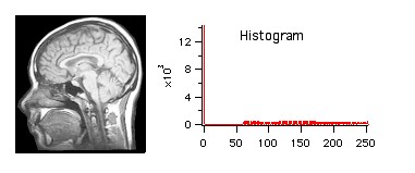
Global histogram equalization and the final gray-scale histogram. Comparing the results with the figure above we can see that the distribution was shifted towards higher values while the peak at minimum intensity remains.

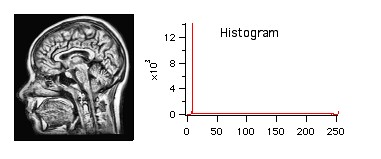
Adaptive histogram equalization shows better contrast over different parts of the image. The corresponding gray-scale histogram lacks the mid-levels present in the global histogram equalization as a result of setting a high contrast level.

A much more common complication involves color images. Here a straightforward histogram equalization on each one of the color channels will lead to color shifts. A better way of modifying histograms for color images is to convert the image into another color space (see Color Spaces), apply the histogram modification to the luminance channel and then convert the image back to RGB.