The test provides a measure that indicates the fit of the distribution of your data to some known distribution. To illustrate how it works we start by generating 1000 pseudo-random data points with a Gaussian distribution:
Make/N=1000 data1=10+gnoise(10)
Although it is not necessary for the purpose of the test, we compute the cumulative distribution function for this data set using the following commands:
Make/N=16/O W_Hist;DelayUpdate
Histogram/P/B=4 data1,W_Hist
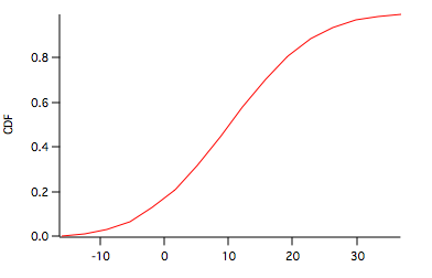
Integrate/METH=1 W_Hist/D=W_INT
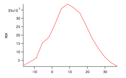
Here W_Hist is the PDF shown above and W_INT is the CDF shown below.
To compare this to a normal CDF we can use the built-in StatsNormalCDF in the following user function:
Function getUserCDF(inX)
    Variable inX
    return statsNormalCDF(inX,10,10)
End
To run the KS test execute the command:
StatsKSTest/T=1/CDFF=getUserCDF data1
Note that the operation's input are the raw data and a user defined continuous distribution function. The results are shown in the Kolmogorov-Smirnov Test table:
| alpha | 0.05 |
| N | 1000 |
| D | 0.0184245 |
| Critical | 0.0427766 |
| PValue | 0.501019 |
Since the test statistic D is smaller than the critical value we can't reject the null hypothesis that the two distributions are the same.
To illustrate a difference between distributions, suppose your data have a Poisson distribution as in:
Make/O/N=1000 data2=poissonNoise(10)
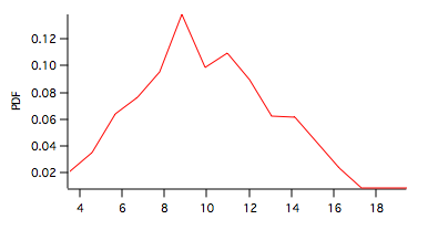
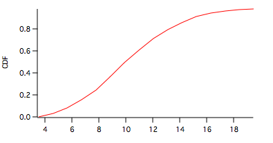
Here the PDF is shown in the graph above and the CDF below.
To test this data set against the same normal distribution as above you can execute the command:
StatsKSTest/T=1/CDFF=getUserCDF data2
which yields the following table:
| alpha | 0.05 |
| N | 1000 |
| D | 0.286538 |
| Critical | 0.0427766 |
| PValue | 1.80085e-73 |
In this case the test statistic D is clearly larger than the critical value and the hypothesis that data2 is taken from a normal distribution is rejected.

Forum

Support

Gallery
Igor Pro 10
Learn More
Igor XOP Toolkit
Learn More
Igor NIDAQ Tools MX
Learn More