The ImageInterpolate operation covers a broad range of interpolation techniques that apply to different types of data. If you are starting from scatter data, i.e., data that is sampled on a non rectangular grid, your choices for interpolation are to use Kriging or Natural Neighborhood Interpolation.

Natural Neighborhood Interpolation

This type of interpolation applies to X, Y, Z, data where the X and Y values describe arbitrary points in the Z=0 plane. The interpolation is valid only for the convex domain containing the data. The algorithm first computes the Delaunay triangulation in the Z=0 plane and then uses the associated Voronoi polygons to interpolate the Z-value for any other point in the domain.

Scatter Data Example

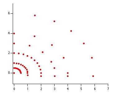
The XY locations in the plane Z=0

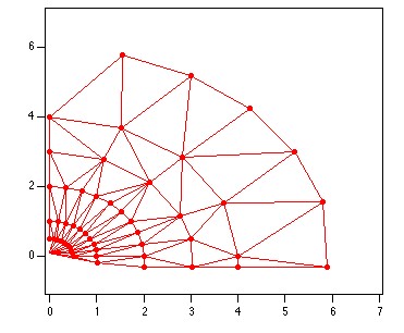
The Delaunay triangulation of the data.

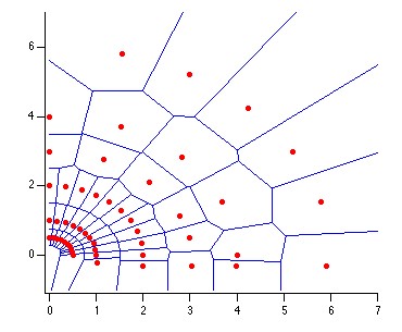
The Voronoi polygons corresponding to the Delaunay triangulation.

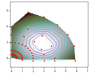
The interpolated image with red markers showing the positions of the data and contour lines going through isolevels.

Kriging

Kriging is an exact interpolator obtained by minimizing variances with a user selected variogram model.

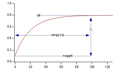
Classic shape of a variogram models showing the nugget, the sill and the range.

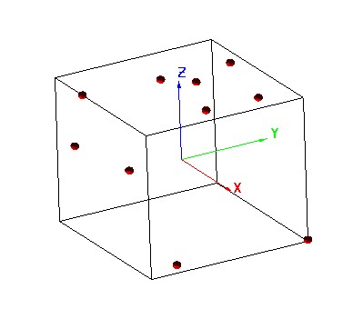
Original data shown as small spheres in a Gizmo plot.

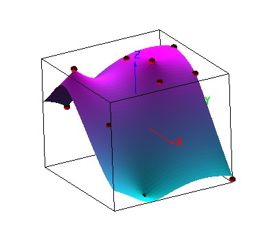
Interpolated surface using kriging and a "spherical" variogram model.

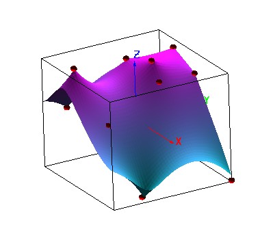
Interpolated surface using kriging and an "exponential" variogram model.

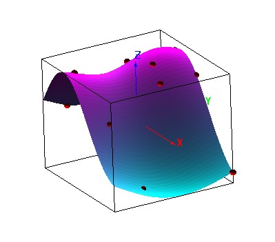
Interpolated surface using kriging and a "Gaussian" variogram model.

Reference: P.A. Burrough and R.A. McDonnel, "Principles of Geographical Information Systems", Oxford, 1998.

If your data is sampled on a rectangular grid, you can use ImageInterpolate to resample it using bilinear, spline, cubic and sinc interpolation. You can also use the operation to warp images or to correct them for certain optical aberrations.

Image Warping

In the following example we perform manual warping of the Lena image.

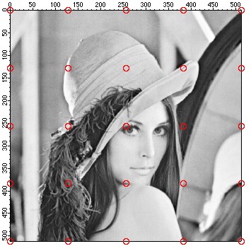
The Lena image with a superimposed regular grid drawn as red markers.

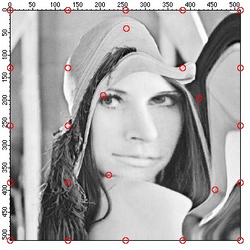
The warped image. Note that the grid points (red markers) have been shifted compared to their position in the original image

Reference: G. Wolberg, "Digital Image Warping", IEEE 1990.

Image Resampling

The ImageInterpolate operation supports various forms of resampling. These might be useful, for example when you want to scale an image. The simplest interpolation method for resampling is called the "nearest neighbor" where a pixel in the output image is computed as the value of the nearest mapped pixel in the source image. Since there is little calculation involved in this interpolation method, it is the fastest. The next resampling method is the bilinear interpolation where the destination pixel is computed by combining the linear interpolation along two orthogonal axes. Although this interpolation method produces smoother results than the nearest neighbor approach, the results for sharp transitions are not ideal. Smoother results and anti- aliasing can be accomplished with spline, cubic polynomial and sinc interpolation considered as more "expansive" mthods as they tend to require more computation as they involve more data points from the surrounding neighborhood.

Smoother interpolation results are not always desirable, e.g., when you scale a binary image or when you need to maintain high contrast for subsequent operations susch as edge detection. Furthermore, the sinc interpolation and to an extent also the cubic interpolation involve a larger neighborhood around the immediate pixel value. This sometimes results in ringing or a tail around sharp edges as we illustrate below.

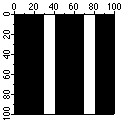
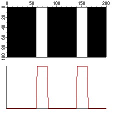
2X horizontal scaling using cubic interpolation. The line profile below the image shows a fairly sharp transition.

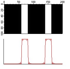
2X horizontal scaling using sinc interpolation. The line profile below the image shows a noisy transition that is also evident by close examination of the image.

Digital Image Correction

Two of the most common problems present in high resolution digital images are distortion (when using wide angle lens) and chromatic aberration. ImageInterpolate can be used to correct for both.

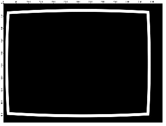
This is a synthetic image showing a barrel distortion of a rectangular frame.

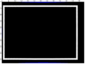
Corrected image shows a square frame. Note that the final image will require some cropping because the areas shown in blue do not correspond to any pixels in the source image.

Correcting chromatic aberration

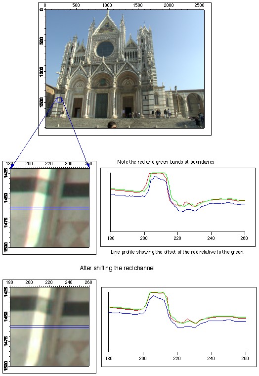
Chromatic aberration is caused by lens systems where the compensation for the dispersion of glass is imprefect at some lens settings. The aberration results in different wavelengths being refracted slightly differently and it can be observed on the image as green and red fringing along intensity boundaries. You can use the ImageInterpolate operation to correct such images by selectively offsetting in the radial direction the corresponding color channels. In the example below an RGB image of the Cathedral in Siena shows under magnification approximately 1 pixel radial offset in the banding of the red and green pixels along the transition border. The corresponding line profile on the right clearly shows the red channel offset. Using ImageInterpolate ReSample with bilinear interpolation and radial polynomial transformation we offset the red channel as shown in the lower line profile.