If you have spectroscopic, chromatographic or other forms of data containing multiple, often overlapping peaks, you will appreciate Igor Pro®'s multi-peak fitting package. This package, like many others included with Igor, can be accessed simply by choosing a menu item.

• Fit any number of peaks in one data set.
• Work on multiple data sets simultaneously.
• Fit six different peak types provided with the package.
• Fit six different baseline types.
• Mix different peak types in a single fit.
• Automatic peak finder.
• Graphically add and edit peaks.
• Location, FWHM, peak height, and area for fitted peaks.
• Can compute FWHM, location, etc. even when there is no analytic expression.
• Write your own peak and baseline functions.
• Support for Igor programmers to use the fitting engine.
• Support for Igor programmers to do batch peak fitting.

To start, you select Start New Multi-peak Fit from the Analysis menu. In the resulting control panel, choose your x and y data.

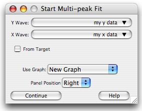
When you click Continue, the result is a graph with an associated control panel "stuck" to the graph. This control panel controls most aspects of choosing peak types and generating initial guesses. You can have as many different graphs and data sets under analysis simultaneously as you want since each graph has its own control panel.

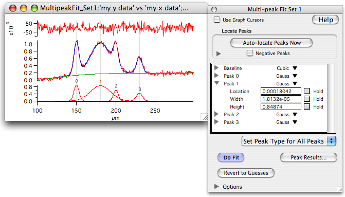
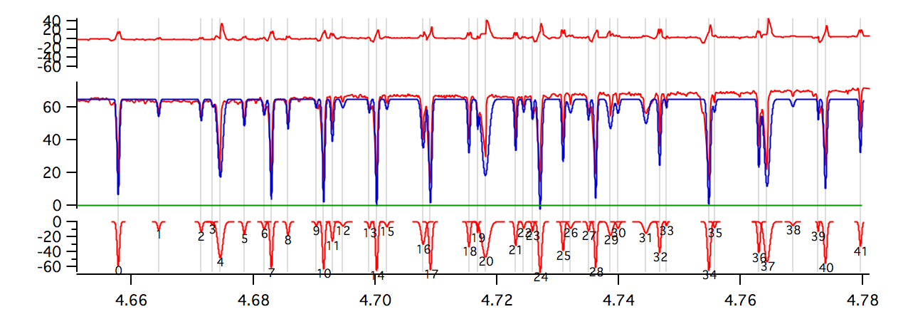
Individual peaks, the overall fit trace and baseline are included on the graph. The residuals plot (at the top in the graph above) is very handy in deciding whether the fit is good or whether there may be additional peaks lurking in the data. In the result shown above the residuals are just noise indicating a good fit.

Note: fitting to overlapping peaks has often been called "deconvolution." This is not strictly correct as the peaks are merely added together and not convolved in the mathematical sense.

Peak types

This package can fit multiple overlapping peaks using any of six basic peak fit types: Gaussian, Lorentzian, Voigt, ExpModGauss, ExpConvExp and LogNormal. The ExpModGauss function is also known as Exponentially Modified Gaussian. You can use any mix of these peak types while fitting a single data set. The following graph illustrates the different types:

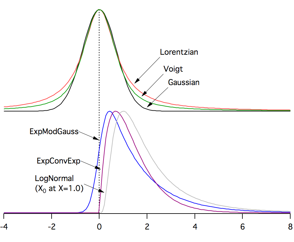
The various peak types shown here (except LogNormal) have been adjusted to have the same Full Width at Half Max. All the peaks except LogNormal have their location parameter set at zero.

A Voigt is the convolution between a Gaussian and a Lorentzian. It includes a shape parameter that adjusts the relative contribution of the two. A shape factor of zero is pure Gaussian with the Lorentzian contribution increasing as shape increases. A Voigt is often used in spectroscopic and X-ray work.

ExpModGauss is the convolution between a Gaussian and an exponential decay while ExpConvExp is the convolution of two exponential decays. The three asymmetric peak shapes can be useful in fitting chromatographic data.

Baseline

The package supports a variety of baseline functions, including none, a simple vertical offset, linear, and cubic polynomial. In general, it is much better to fit with a baseline function than to try to remove the baseline from the data and then fit. However, especially in cases where there is a clear distinction between baseline and peaks, you can use any other Igor capabilities to subtract out the baseline before the fit.

User Peak and Baseline Functions

The Multi-peak Fit package has peak types and baseline functions that will answer most needs. If you cannot find an appropriate peak type or baseline function, you can extend the package by writing your own functions in Igor's internal language.

Setting initial values

The initial values for the fit, i.e., the number, placement and properties of the peaks, can be set in several ways. You can enter values numerically, use the auto peak finder, interactively draw or edit your peaks with the mouse or some combination of these methods.

Using AutoFind

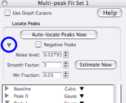
Usually you will start the analysis of a data set by clicking the button labelled "Auto-locate Peaks Now". This invokes an automatic peak-finding algorithm that searches for peaks by finding maxima in the smoothed second derivative of the data. The algorithm tries to guess the noise level of your data and, most critically, an optimum smoothing factor used on the second derivative of the data.

If the fully automatic peak finder does not work for your data, you may be able to get better results by adjusting parameters used by the auto peak finder algorithm. You get access to the settings by clicking the arrow in the Locate Peaks box:

In particular, if your peaks are narrow, you may need to reduce the smoothing factor. This data set is best handled using a smoothing factor of 1:

This is also an example of the ability to find and fit negative peaks. In this case, the Negative Peaks checkbox was turned on; the auto peak finder can't automatically detect the polarity of peaks.

Using Manual Peak Adjust

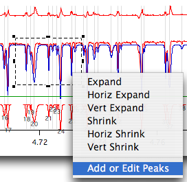
If the automatic peak find does not work for you or if you need to make adjustments to the peaks before fitting, drag out a marquee on the graph and select Add or Edit Peaks from Igor's marquee menu:

The resulting Add or Edit Peaks graph allows you to delete a peak, insert a new peak or edit an old peak. As you point the mouse at an existing peak curve, the trace on the graph is highlighted. In this picture, the cursor is highlighting Peak 20:

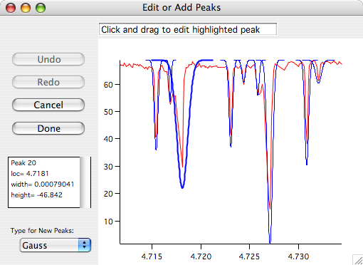
When a peak trace is highlighted, you can click and drag to change the width, height or location of the peak. Or you can right-click and select Remove to delete a peak.

To add a new peak, simply click in an area where no existing peak trace is highlighted. The top of the peak will be at the initial click location; drag to set the height and width. You can add as many new peaks as you wish. If you put one in the wrong location, you can simply point, click and drag to adjust it.

If you don't like what you've done, click the Undo button. A complete record of actions in the Add or Edit Peaks graph is kept, so that you can undo any actions taken. If you undo too much, you can click the Redo button.

When you are finised adjusting, adding or deleting peaks, click the Done button. The main peak fitting graph and the list of peaks in the control panel will be updated to reflect your changes, and a new fit curve and new peak traces will be drawn.

Fitting to sub-ranges

For some data sets, it is more efficient to fit several subsets of your peaks rather than trying to fit everything at once.

There are two ways to limit the range of data included in a given fit. You can set the range of data shown in the graph by zooming in on just the data of interest. By default, the Multi-peak Fit panel works on all the data showing in the graph.

You can also place graph cursors on the graph, and turn on the checkbox Use Graph Cursors. Multi-peak Fit will now fit only the data between the cursors.

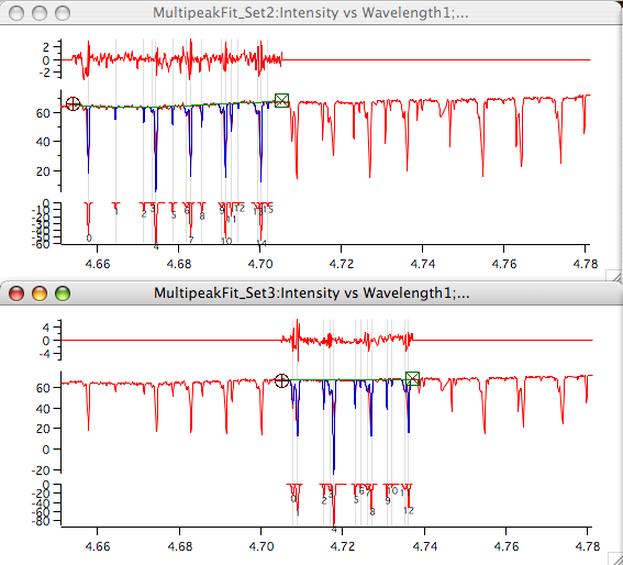
At this point, you could just move the cursors to another part of the graph and do another f it. But you would lose the results of the first fit. So now you can go back to the Start New Multi-peak Fit panel, select the same data set as before, and make a new Multi-peak Fit graph. Set the cursors to the new range, and do another fit.

Here is a picture of two graphs of one data set, each with a fit to a different portion of the data:

Creating fit results

After a successful fit, you can get a variety of results from the fit by clicking the Peak Results button. When you do that, a table is created containing a summary of the peaks. The table includes the real location of the peak, the real amplitude, the area and Full Width at Half Maximum (FWHM) for each peak, as well as the basic fitted coefficients and estimates of errors for each quantity.

In some cases, such as the real location of a ExpModGauss peak, there is no analytic expression. For those results, Multi-peak Fit uses a numeric method to find the needed information. In that case, the error estimate is not available.

Included in the window containing the table of results are three buttons: Report in Notebook, Graph, and Standard Parameters, Tab Delimited. These buttons give you a nicely formatted document suitable as a report on the fit, or the starting point for a publication graph showing the fit, or a tab-delimited file that could be imported into another program.