Mathematical transformations of images may be as simple as image arithmetic or as complex as an iterating Fourier transform. You can handle most image arithmetic by executing Igor Pro® commands. For example, to subtract a background image:

Duplicate noisyImage,outputImage

outputImage=inputImage-backgroundImage

When working with images that are 8 or 16 bit per pixel you can perform level mapping using

outputImage=LUT[inputImage[p][q]]

here LUT is a lookup table for the mapping. For example, LUT can be used for Gamma correction using an expression like

LUT=p^(1/Gamma)

Most arithmetic operations are performed more efficiently using MatrixOP.

Fourier Transforms

The Fast Fourier Transform (FFT) can be used to decompose a grayscale image into its spatial frequency components or to perform efficient 2D convolutions and correlations (RGB images are usually handled on a channel by channel basis).

In the following example we illustrate simple FFT filtering. We created an image that consists of a one dimensional slow quadratic ramp and added single frequency sinusoidal noise. The filter consists of a 2D constant wave with a single null pixel. The filtering consists of a single command line:

MatrixOP/o filtered=IFFT(filter*FFT(inputImage,2),3)

​

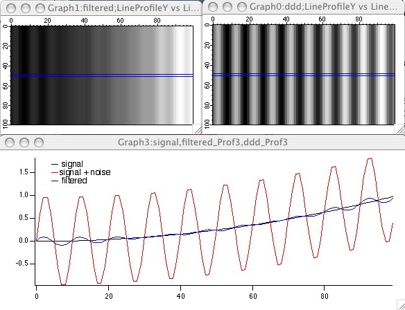
The input is shown on the top right, the filtered image is shown on the top-left. The blue lines mark the position of measured line profiles which are displayed below the images.

After an image has been filtered by convolution with some filter, it is not always possible to recover the original from the filtered version. One approach for deconvolution is known as a Wiener filter:

Create the Gaussian blur filter

Make/O/N=(512,512) blur=exp(-((x-255)/9)^2-((y-255)/9)^2)

Perform the convolution and add uniform noise

MatrixOP/O blurredImage=IFFT(FFT(lena,2)*FFT(blur,2),3)
ImageTransform swap blurredImage
blurredImage+=enoise(2)

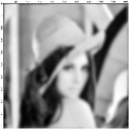
Lena's picture using a Gaussian blur and uniform additive noise.

The Wiener filter has the form:

Estimated Image = O*Hc/[H*Hc+ fn/fs]

where O is the Fourier transform of the convolved image, H is the Fourier transform of the convolution filter, Hc is the complex conjugate of H, and fn/fs is the ratio of the noise to signal power spectra. The Weiner filter is designed to minimize the mean square error of a linear estimate. The difficulty of applying the filter is in finding the appropriate values for fn/fs since the noise is not usually known. In practice one can frequently replace fn/fs with a constant value that applies over the whole image or try to estimate the value on a region by region basis.

MatrixOP/O estimated=IFFT(FFT(blurredImage,2)*h/(h*hc+0.04),3)
ImageTransform swap estimated

​

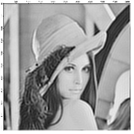
Recovered image using Wiener filtering.

The Wavelet Transform

The wavelet transform is used primarily for smoothing, noise reduction and lossy compression. In all cases the procedure is to first perform a forward wavelet transform, then perform some operation on the transformed image followed by an inverse wavelet transform. In wavelet compression, for example, the compressed image is the part of the transform that corresponds to the low order coefficients in the transform (similar to low pass filtering in 2D Fourier transform). The reconstructed image exhibits a number of compression-related artifacts, but it is worth noting that unlike an FFT based low-pass filter, the advantage of the wavelet transform is that the image contains a fair amount of high-frequency content.

To illustrate the application of the wavelet transform to de-noising, we start by adding artificial noise to an image:

Mri+=gnoise(10)		 

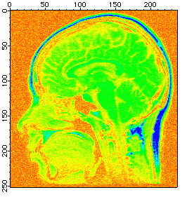
To denoise the image we use:

DWT/D/N=20/P=1/T=1/V=0.3 Mri,dMri	 // increase /V for more denoising

​

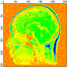
The denoised image showing significant noise reduction at the cost of minor wavelet transform artifacts.

Hough Transform

The Hough Transform is a mapping algorithm in which lines in image space map to single points in the transform space. It is most often used for line detection. Specifically, each point in the image space maps to a sinusoidal curve in the transform space. If pixels in the image lie along a line, the sinusoidal curves associated with these pixels all intersect at a single point in the transform space. By counting the number of sinusoids intersecting at each point in the transform space, lines can be detected. Here is an example of an image that consists of one line.

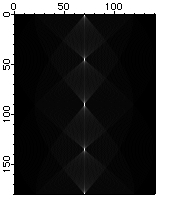
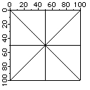
The source image shows a series of bright pixels in the center. The first and last points are transformed into lines at 0 and 180 degrees. The second point from the top corresponds to the line at 45 degrees and so on.

Hartley Transform

The Hartley transform is similar to the Fourier transform except that it uses only real values. The transform is based on the cas kernel defined by:

	cas(vx) = cos(vx) + sin(vx).

The discrete Hartley transform is given by

The Hartley transform has two interesting mathematical properties. First, the inverse transform is identical to the forward transform, and second, the power spectrum is given by the expression:

The implementation of the Fast Hartley Transform is part of the ImageTransform operation. It requires that the source wave is an image whose dimensions are a power of 2.