Convergence problem with Shirley background All-at-once-fit


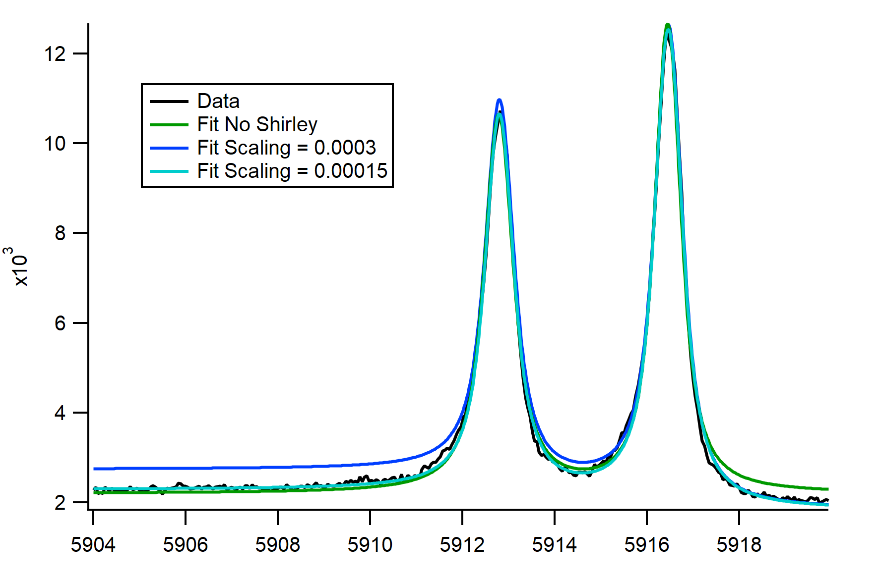
I am trying to fit XPS data with a custom all-at-once fit function and while the basic fit generally seems to converge to the extend the model allows, adding a Shirley background (based on the model wave) shows unexpected behaviour. I used a scaling factor to resize the background, which turns out to be way off. I attached an image showing the original converged fit, the converged fit with a Shirley background and a fit with identical fit parameters but adapted scaling factor. In the shown case the scaling is about a factor of two too big, in a different case (fit with Doniach-Sunjic lineshapes) it was about 2.5 times too small. All other parameters seem to still converge somewhat reasonably though in the second case the amplitudes were comparably well fitted but the numbers unexpectedly changed. Any advice would be appreciated.
The fit function I use is based on others I found and adapted. Feel free to give advice for improvement independent of solving the problem. I'm working in Igor 8.04. The fit function is this:
// Amplitude-normalised Gauss profile
//------------------------------------------------------------------------------
Function Gauss(x_val, offset, amplitude, peakpos, fwhm)
//------------------------------------------------------------------------------
	variable x_val, offset, amplitude, peakpos, fwhm
	variable sigma = fwhm/(2*sqrt(2*ln(2)))
	return offset + amplitude*exp(-(x_val-peakpos)^2/(2*sigma^2))
End


//------------------------------------------------------------------------------
Function Voigt2S_fit(pw, yw, xw) : FitFunc
//------------------------------------------------------------------------------
	WAVE pw, yw, xw

	//CurveFitDialog/ Equation:
	//CurveFitDialog/ f(x) = L1+L2+shirley+offset
	//CurveFitDialog/ End of Equation
	//CurveFitDialog/ Independent Variables 1
	//CurveFitDialog/ x
	//CurveFitDialog/ Coefficients 9
	//CurveFitDialog/ pw[0] = Constant_background
	//CurveFitDialog/ pw[1] = Scaling_Factor_Shirley
	//CurveFitDialog/ pw[2] = Gaussian_broadening_FWHM_eV_instrumental)
	//CurveFitDialog/ pw[3] = L1__Amplitude
	//CurveFitDialog/ pw[4] = L1__Position_eV
	//CurveFitDialog/ pw[5] = L1__FWHM_eV
	//CurveFitDialog/ pw[6] = L2__Amplitude
	//CurveFitDialog/ pw[7] = L2__Position_eV
	//CurveFitDialog/ pw[8] = L2__FWHM_eV


	variable RangeIncreaseFactor = 5							// if G_FWHM=0.1eV, output wave spans RIF*0.1eV
	variable oversampling = 4
	variable xdeltaNew = DimDelta(yw,0) / oversampling	// xw resolution of the fit wave


	// ---------- Broadening Wave -----------
	variable fwhmB = pw[2]													// in eV
	variable xhalfB = (1/2) * fwhmB * RangeIncreaseFactor			// half energy range of wave
	variable nbxValB = 2 * floor(xhalfB / xdeltaNew) + 1

	variable nbxValRef = DimSize(yw,0)*oversampling					// "regular" size of the model without broadening addition
	nbxValB = min(nbxValB, 2*nbxValRef)									// limit the resolution of broadening
	Make/D/FREE/N=(nbxValB) broadening
	SetScale/P x -xhalfB, xdeltaNew, "", broadening
	broadening = Gauss(x, 0, 1, 0, fwhmB)							// Gauss of amplitude 1
	variable sumB = sum(broadening, -inf,inf)
	broadening /= sumB


	// ---------- Model Wave ----------------

	// Extend the model area by half a Gaussian to avoid deconvolution effects
	variable xminM = DimOffset(yw,0) - xhalfB
	variable xmaxM = DimOffset(yw,0) + DimDelta(yw,0)*DimSize(yw,0) + xhalfB
	variable nbxValM = floor(abs(xmaxM-xminM)/ xdeltaNew) + 1

	Make/D/FREE/N=(nbxValM) model
	setscale/P x xminM, xdeltaNew, "", model

	// ---------- Peaks ---------------------
	model = LorentzForDS(x, 0, pw[3], pw[4], pw[5])
	model += LorentzForDS(x, 0, pw[6], pw[7], pw[8])			// x, offset, amp, pos, fwhm


	// ---------- Convolution ---------------
	Convolve/A broadening, model


	// ---------- Background ----------------
	Make/D/FREE/N=(nbxValM) shirley_bg
	setscale/P x xminM, xdeltaNew, "", shirley_bg
	shirley_bg = 0

	variable j
	for(j=nbxValM-2; j>-1; j-=1)								// -2 accounting for start at 0 and avoid max due to j+1
		shirley_bg[j] += shirley_bg[j+1] + model[j]
	endfor

	shirley_bg *= pw[1]


	// ---------- Model ---------------------
	model = model + shirley_bg + pw[0]

	yw = model(xw[p])
End
From a quick review of your procedure, I would ask these questions:
* As I recall, a constant baseline can be used to set the low BE side (high KE side) to zero before the fitting. Why not remove this constant before the fitting process rather than including it as a parameter in the fit function?
* As I recall, when I created a Shirley baseline, I used the integrate operation working from the low BE (high KE) side. Why are you doing a summation in a for-endfor loop?
* As I recall, after I integrated the curve to obtain the Shirley baseline, I then scaled the integral baseline curve so that its two extreme end points fit to the baselines of the raw data at the two extreme end points. Why are you using a variable scaling factor at all?
September 12, 2020 at 09:28 am - Permalink
In reply to From a quick review of your… by jjweimer
anHi, thanks for the reply. To your questions:
* I did not consider subracting a baseline early on because with the noise I did not see a proper way to determine it. Plus, I hoped it would implicitly be taken care of in the subsequent iteration steps. This goes hand in hand with the answer to question three:
*** I have some spectra with strongly asymmetric peaks leading to an overlap of the tails and background at the high BE end of the spectra. Thus I was hoping a flexible fitting that was not attached to the x axis extreme points would allow for a more correct determination of the asymmetry.
The above does not seem to have a major effect but I might oversee something here.
** You are totally right. I suppose the main problem was a wave-scaling caused normalisation issue in the summation. I replaced it with the integration and the scaling problem seems solved. However, I tried to yield the inverted integration by use of the Reverse function but the integration seems to go after the x values. I worked around that by using negative numbers but it's not pretty and slowed the fitting considerably. Another hint on that?
September 12, 2020 at 10:55 am - Permalink
To your responses:
* To remove a constant on noisy data ... Average the values for a few points (1-5) at the lowest BE. Subtract that average value. Alternatively, find the minimum value of the data set. Subtract it. Either method will obtain a reasonable input to the fitting routines without having to remove a constant within the fitting routines themselves.
* When you have additional peaks (e.g. plasmons) or features (tails from peaks) that contribute at high BE, you have two options. You can record the XPS spectra to a higher range of BE to allow your experimental data to become purely the baseline. Alternatively, you can incorporate the additional peaks or features directly in the fitting routine itself. To be honest, based on what you show for the "best fit", I see no reason that you should not be able to set the Shirley baseline as the only contribution at BOTH the lowest BE position AND at the highest BE position. I do not see significant contributions from "tails" at high BE.
* Yes, you must remember that integration should consider the wave scaling. The best way that I recall is to set all waves (fitting waves and the Shirley background wave) to the same x-scaling as the raw data.
Some other thoughts:
* You can avoid the need to SetScale multiple times. Just Duplicate your raw wave to the Shirley baseline and model. The x-scale will be preserved.
* You should remove the constant background outside the fitting function.
* I believe that a viable alternative approach to using negative x scaling for an integration is to multiply the resultant wave value by -1 after integration. Or to shift it and then multiply. I recall that I had to graph the waves at each step and figure it out using the shapes of the curves and their scaling. I also recall that I did NOT scale the Shirley baseline going negative to get what I needed.
September 12, 2020 at 11:29 am - Permalink
You can include the Shirley background in the fit either analytically or by numerically integrating the model wave in your fit functions. You went with the numerical integration approach.
I used the analytical approach. For symmetric pseudo Voigt peaks described as a sum of a Gaussian and Lorentzian peaks, the Shirley background is the sum of the two integrals given by ArcTan and Erf. If you want to use this approach for asymmetric peaks you need to known the integral of the asymmetric peak. Because of that I use an asymmetric peak shape made up of a sum of symmetric peaks, but there are many other solutions to this.
Below you can find a simplified version of what I do in my EccentricXPS procedure. I am showing the code not optimized for speed (I use it for testing because it is easier to understand what it does) and I removed the asymmetric part.
September 13, 2020 at 03:35 am - Permalink
I did not use the built-in Gauss function because I want to be able to define and constrain peak areas
September 13, 2020 at 03:40 am - Permalink
In reply to To your responses: * To… by jjweimer
an@jjweimer
*I went back to the baseline effect and was trying to get a subtraction of wavemin() to work, as you proposed, which also yielded good results when subtracted prior to fitting. However, I could not find a way to manipulate the handed in data wave from within the fit to allow for use of the curve fit dialog and still maintaining a single fitting step (though it seems the offset parameter used before matches the wavemin() value closely)
* For this spectrum that is indeed true but I would like a single function to use for all my data. Unfortunately, most spectra are not very 'clean' and increasing the energy range would be a never ending process. Thus the preverence for a flexible background.
* As far as I see the scaling is consistent for the model and was increased in comparison to the data for the convolution (?) and to allow having nicely resolved fits for low-resolution data. It seems Igor is handling the projection on the different scaling at the end of the iteration quite well.
* I was clearly confused about the sign changes coming with the inversion. In the end, reverse was the correct approach:
I suppose this is the multiplication by -1 that you were talking about.
September 13, 2020 at 05:46 am - Permalink
In reply to You can include the Shirley… by olelytken
anHi olelytken,
thanks for the code. At the moment I am using Doniach-Sunjic lineshapes (infinite area) and would to prefer to keep it this way for now. But I'll keep it in mind.
September 13, 2020 at 05:55 am - Permalink
With regard to your comments:
* You can now either remove one fitting constant (the offset) or use a HOLD string to keep that offset value pinned at zero during the fit. I would personally recommend the former approach. Establish a pre-process function before the all-at-once fitting that will a) remove the offset and b) generate the first guess Shirley baseline (or generate a zero Shirley baseline). Establish a post-processing function that will add back the offset to the returned waves.
* The trade-off in your approach is that you are allowing flexibility to replace rigor. I'm rather surprised in this case that you take the effort to use the DS line shape yet do not include plasmon peaks and/or set your background to truly go to just the background at higher BE.
* The process of convolution can/does affect the scaling of the resultant wave. This is an entire discussion into itself.
* I would integrate with the trapezoid rule at least. The default is /D=-1, so this flag is not needed. You can just integrate directly into the Shirley background as its own destination (eliminate the need for model_rev or make model_rev a FREE wave). Yes, this is the approach I believe that I took with a negative scaling factor.
Oletyken has good recommendations. In particular, when you are doing the fitting to metal doublets with DS line-shapes, you will want to constrain the peak area ratios for the two spin-split peaks to their theoretical value. When you are not doing this and you are also ignoring the plasmon or loss regions at high BE on your fits, you may as well just go back to Gauss or Lorentz or Voigt peak shapes. The gain in "accuracy" that you may propose to have achieved using DS line shapes for the metal peaks is likely lost in the sloppiness of everything else that you did not do to sustain the true theory.
Apologies otherwise. I digress to a soapbox stand that I once took many years ago doing XPS analysis as a core part of my career. At least you are not fitting two simple Gaussian peaks with no real constraints between them, tacking on a sloping straight line baseline, and calling those end results worthy of publication (as I see even in the literature today).
September 13, 2020 at 09:03 am - Permalink
In reply to With regard to your comments… by jjweimer
an*I'll have a look at your list from https://www.wavemetrics.com/forum/general/rectangular-vs-trapezoidal-in…
*As a newbie to the field and Igor with little to no programming experience, picking the original lineshapes was a choice of ease to get started and figure out the basics. I am aware that the approach has its weaknesses and I appreciate to have had pointed out the flaws. I'll give reworking it another shot in the future.
September 14, 2020 at 07:20 am - Permalink
As a new user to Igor Pro, you've made excellent strides so far. I do recommend that you take a look at the EccentricXPS package that Olelytken has developed. Having created a package for XPS analysis many years ago, I can tell you that the process to get it done right can be a never-ending cycle. You may be better to jump into something that already is robustly developed (EccentricXPS) rather than trying to roll your own from the ground up.
September 14, 2020 at 07:17 pm - Permalink
The procedure I developed, EccentricXPS, cannot do Doniach-Sunjic line shapes and I have no plans to implement them, but I think XPS Tools by Martin Schmid may have Doniach-Sunjic line shapes, if those are important to you.
September 14, 2020 at 11:01 pm - Permalink