Scaling of images


Hi all,
I have two images of the same object, but with different field of view (Field-of-view (FOV) refers the distance (in cm or mm) over which a magnetic resonance image is acquired or displayed), i.e. this object looks small in one image and big in another image. How can I scale these images to make the object have the same sizes in these two images? Please find attached the figure clarifying the problem.

Forum

Support

Gallery
Igor Pro 10
Learn More
Igor XOP Toolkit
Learn More
Igor NIDAQ Tools MX
Learn More
I think you need to know the pixel size for each image and the ratio between them and then do ImageInterpolate with the /TRNS flag to rescale the appropriate image.
April 12, 2019 at 07:40 am - Permalink
If you use wave scaling and then have the X and Y axis share the same respective ranges in both images is another way to have them appear the same.
Note: If you are going to do some image processing those operations work on the pixel not the scaled dimension.
Andy
April 12, 2019 at 07:59 am - Permalink
In reply to If you use wave scaling and… by hegedus
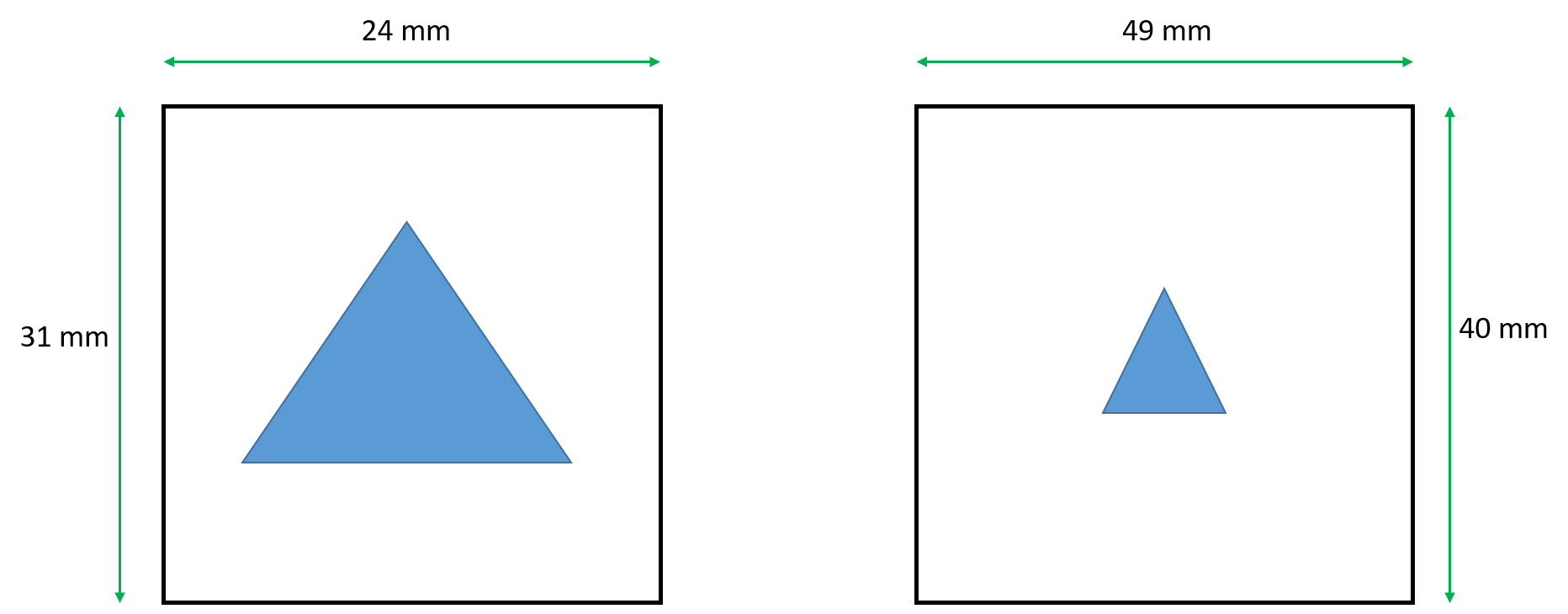
Physicist92I load two images, each of them has matrix 512 x 512. Then I do Data --> Change Wave Scaling, choose SetScaleMode --> Start and Right, Units = mm, and write 24 mm for X, 31 mm for Y, and similarly for the second image (49 mm, 40 mm). So what is the next step? Could you please tell me, what command should I use to make the object have the same sizes in these two images? It is like zooming.
April 13, 2019 at 02:31 am - Permalink
Create two image plots with each wave respectively. Set the X and Y scale range the same for both graphs and make the overall graphs the same size. The features should now appear the same size.
April 13, 2019 at 06:54 am - Permalink
In reply to Create two image plots with… by hegedus
Physicist92Sorry for misunderstanding, but how can I set the X and Y scale range the same for both graphs? If I set X = 24 mm and Y = 31 mm for both images, or X = 49 mm and Y = 40 mm for both images, it will be incorrect, because one image has FOV = 24 mm x 31 mm, and another image has FOV = 49 mm x 40 mm. If I set equal X and Y scale for both images, I will set wrong FOV for one image.
April 13, 2019 at 08:55 am - Permalink
Hi,
There are two scales to set or to be a bit more precise: There is a scale for your data/image and then there is the scale or range of the axis in your graph. The setscale operation allows you to use IP built-in functionality to define the dimensionality of the data. Good.
When you create a graph of your data the default action is to set the axis range to the full scale of your data both in X and Y. Most graphing software does this and it is a best practice. The issue you are facing is that the default scaling of the axis cause a difference in perception. To overcome this issue, the range of the axis in both graphs should be the same. For your example the x axis range should be 0-49 (or 0-50) in both graphs. Likewise the y xis range should be 0-40 for both graphs. And if the overall graph size is the same then the objects should appear to be same size.
There is another way to do this with scaled images though with some limitations. Create a new image graph and then append the second image to that graph taking care to use the same axis (newimage uses a top x axis and reversed y axis). The second image will obscure the first but the x and y axis will now be the same for both. In the image menu there is a reorder image operation to allow you to bring a particular image to the fore. Unfortunately for color images there is no option I have found to hide the other. That is the limitation. With grayscale images you can play some tricks to make an image transparent, but they are not available for RGB image.
I mocked up an experiment to help explain. In it are the original FOV scaled images, the first with x and Y axis to match the range of the second image, and lastly an image plot with both and a popup control to bring a specific one to the front.
Andy
April 13, 2019 at 09:44 am - Permalink
In reply to Hi, There are two scales to… by hegedus
Physicist92Thanks a lot!
April 13, 2019 at 12:21 pm - Permalink
You are welcome.
One nice feature to add to the wishlist is the ability to hide an image in graph. Currently you can hide traces, but not images.
Andy
April 13, 2019 at 01:35 pm - Permalink
In reply to I think you need to know the… by sjr51
Physicist92Hi all,
Could you please explain how to run correctly ImageInterpolate command with /TRNS flag?
For example, I have two images (wave A1 and wave A2): one image (A1) has field of view = 24 mm x 31 mm, and another image (A2) has field of view = 49 mm x 40 mm. Both images have matrix = 512 pixels x 512 pixels. Thus pixel size for the 1st image = 0.046875 mm x 0.060546875 mm. Pixel size for the 2nd image = 0.095703125 mm x 0.078125 mm.
Syntax for ImageInterpolate command is the following:
ImageInterpolate [ flags ] Method srcWave
/TRNS={transformFunc,p1,p2,p3,p4 }
Determines the mapping between a pixel in the destination image and the source pixel. transformFunc can be:
scaleShift: sets image scaling which could be anamorphic if the X and Y scaling are different.
radialPoly: corrects both color as well as barrel and pincushion distortion. In radialPoly the mapping from a destination pixel to a source pixel is a polynomial in the pixel's radius relative to the center of the image.
I think that I should use scaleShift. But I don't understand, how to set p1, p2, p3 and p4 parameters for /TRNS flag. In IgorPro manual, it is only said that p1 is xOffset, p2 is xScale, p3 is yOfffset, p4 is yScale. But what does it mean? If we consider the given examle with two specific images, what values should I put to p1, p2, p3 and p4 parameters?
June 12, 2019 at 04:13 am - Permalink
The scaleShift transformation is designed for linear scaling where {p1, p3} are offsets and {p2, p4} are the scales in the corresponding directions, i.e., the pixels are mapped using the equations:
x'=p1+p2*x
y'=p3+p4*y.
The output image here should have p2*rows by p4*cols (where rows and cols correspond to the input image).
Generally, (x',y') is not going to be an integer so bilinear/nearest-neighbor/cubic/spline/sinc interpolation will be used to compute the new pixel value. It should be clear that wave scaling of the input is completely irrelevant here.
I hope this helps,
A.G.
June 12, 2019 at 07:34 am - Permalink
In reply to The scaleShift… by Igor
Physicist92Thanks a lot! But is there any possibility to make image interpolation in the case described in the main message of this thread, using ImageInterpolate command? I mean, is it possible to perform interpolation given that wave scaling was made? I.e. images' dimensions are in millimeters.
June 13, 2019 at 07:52 am - Permalink
Wave scaling is a convenience that is unhelpful in image processing and in other numerical calculations. I would argue that in some situations you should actually apply default wave scaling (offset => 0 and delta =>1) in order to improve the accuracy of your calculations. This is easy to see if you consider e.g., factors of h_bar (Plank's constant) in the calculations.
Some image processing algorithms assume that pixels are square. If you worry about that aspect then you should also address the issue that interpolation typically corresponds to the value at the center of the pixel while wave scaling may refer to the edge.
In reference to the OP on this thread, I'd expect to know what one wants to do with the data. For example, if it is expected to be used for any sort of measurement, I would recommend initial interpolation of the data onto square pixels. This would allow you to measure accurate distances in directions that are not parallel to the axes. Also, if you need to rotate the image so that the edge of the object is parallel to the frame you may face additional difficulties.
You can get to square pixels using ImageInterpolate with the /F={fx,fy} flag. I will assume that the right example is 49x40 in which case I'd use fx=1 and fy=(49/40).
I hope this helps,
A.G.
June 13, 2019 at 09:02 am - Permalink
OP: Please re-post your last response together with the attachments.
It is not clear to me why you need to match the different projections and specifically what you mean by "matching". If you are trying to reconstruct the object from the various projections I imagine that you would want the data to use the same scales regardless of FOV.
Unless I am missing something, since you appear to use wave scaling, you can follow:
1. Decide on output resolution and create an output wave with appropriate scaling.
2. Run a loop or make a wave assignment that fills each pixel of the output wave with an interpolated value from the appropriate projection e.g.,
outputWave=Interp2D (projectionWave, x, y )
Note that you might also be able to use ImageRegistration for matching image sizes.
If this does not work for you for some reason, feel free to send a copy of your experiment to support@wavemetrics.com.
A.G.
June 14, 2019 at 07:05 am - Permalink
In reply to OP: Please re-post your… by Igor
Physicist92My last response:
It is magnetic resonance imaging (MRI) (tomography) experiment. There are 3 different images of the same sample (sample is the object which was scanned in MR scanner). These 3 images are 3 orthogonal projections: plane (X-Y), plane (Z-X), plane (Z-Y). There was no slice selection during MRI experiment, i.e. each projection represents the sum of all anatomical slices of the sample in specific direction. I.e. the projection (X-Y) is the sum of all anatomical slices along Z axis: Z1, Z2, Z3, ..., Zn. The projection (Z-X) is the sum of all anatomical slices along Y axis: Y1, Y2, Y3, ..., Yk. The projection (Z-Y) is the sum of all anatomical slices along X axis: X1, X2, X3, ..., Xm. Each projection (image) was loaded into IgorPro as 512 x 512 matrix (wave). Then "Modify Image Appearance" was applied (Geo). After that, wave scaling was applied according to known field-of-views (FOVs) of each image. The first image (projection) has FOV = 20 mm x 30 mm. The second image (projection) has FOV = 50 mm x 40 mm. The third image (projection) has FOV = 43 mm x 35 mm. All these numbers for FOVs are arbitrary but they reflect the essence of the problem: each projection (image) has its own FOV which can be different from FOVs of two other projections (images). Finally, in IgorPro, Aspect ratio was applied in order to show real ratio between sides of an image. Thus pixels are not square after applying Aspect ratio.
In the images, dark blue area is noise area (see the attached picture). In noise area, intensity values should be zero, but actually they are not zero, so in each projection I will have to select ROI covering the whole sample and cut it. The result will be the sample, and the noise will be zero around the sample. So in the picture attached, it is assumed that the intensities in the noise area are already set to zero.
As one can see from the pictures, the sample is non-uniform (three different colors demonstrate this non-uniformity).
I need to divide the intensity in each point of the sample in the left image (X-Y projection) by the corresponding length, i.e. I need to obtain normalized left image. The length for each point should be calculated from the middle image (Z-X projection). Each point (pixel) in the left image is a parallelepiped that is defined by three sides: side1=0.0390625 mm (see attached picture, pixel size under the left image), side2=0.05859375 mm, side3=Length. Lengths are in millimeters. In the attached picture, in the left image, vertical lines are drawn which pass through the sample: X1, X2, ..., Xm (these X values are in millimeters). On each line (X1, X2, ..., Xm), in the interval within the sample, violet points are drawn. The number of violet points on each line is the number of pixels belonging to the sample on this specific X-line. Since there was no slice selection in the MRI experiment, I assume that for each violet point on specific X-line (i.e. for each violet point in specific column of left image), the length is the same.
In the middle image (Z-X projection), horizontal lines are drawn which pass through the sample: X'1, X'2, ..., X'm (these X' values are in millimeters). All points on each X'-line, which belong to the sample, should be considered to calculate lengths: L1, L2, ..., Lm. Length = (number of pixels which lie on specific X'-line and belong to the sample) multiplied by (pixel size along Z axis in Z-X projection).
It seems that the third image (Z-Y projection) is not necessary for calculation.
The problem is that FOVs of the first and the second projections are different. And thus X1, X2, ..., Xm are not equal to X'1, X'2, ..., X'm. I need to match the first and the second image (and maybe all three images, but at least two images). The first variant is to extend the side along X axis in the left image (X-Y projection) from 20 mm to 40 mm. The second variant is to compress the side along X axis in the middle image (Z-X projection) from 40 mm to 20 mm. Which variant would you recommend? And how can I implement this extension (or compression)? Or maybe there is another way to achieve the goal?
New response:
I don't need to reconstruct the object from the projections. The purpose is to obtain normalized left image (normalization factor is length which is different for each pixel in the left image). It is preparation step for further quantitative analysis. (Length should be calculated from the middle image as shown in the attached picture)
Regarding matching. I need to perform matching of the left and middle projections, since I need to know what length should I take for violet points on X20-line in the left image (for example). If the scaling for the side along X-axis in the left and in the middle images were the same (for example, horizontal side = 20 mm in the left image, and vertical side = 20 mm in the middle image), then it would be possible to say that for the violet points on X20-line in the left image, the length can be calculated based on the number of pixels along horizontal X'20-line in the middle image (in this case, X'20 would be equal to X20).
Please find attached the synthetic experiment file. There is procedure code in this file.
June 14, 2019 at 10:25 am - Permalink
It is good to see real examples:
If I understood the problem correctly then I would expect to be able to match two of the images for each axis. For example, I should be able to match the z-axis between graph1 and graph2 using the minimum and maximum extent of object along the horizontal direction. The range of data from the two graphs is different. Graph1 shows the z object range to be 4.78 to 39.16 while Graph2 gives 2.43 to 39.05. I get these values using the Line Profile dialog in IP8 with a horizontal profile and checking the Show Cursors checkbox at the bottom left.
At this point you need to choose which image (of the pair) you want to use as your "key" image. You would then compute the transform for the other member of this pair along one axis to match the key image. The transformation is linear; x'=a*x+b. You have two equations for two unknowns (a and b).
If you repeat this process for the other axes, i.e., use Graph0 and Graph1 for the X range and then use Graph0 and Graph2 for the Y range you should be able to get the transformation coefficients that will allow you to scale two of the images to the key image.
I hope this helps.
A.G.
June 14, 2019 at 10:56 am - Permalink
In reply to It is good to see real… by Igor
Physicist92"Graph1 shows the z object range to be 4.78 to 39.16 while Graph2 gives 2.43 to 39.05."
I checked it using Line Profile in IP8 and cursors, and obtained the following:
Graph1: from 4.78516 to 43.9453 mm (maximum range for the object, i.e. central part). Thus Length = 43.9453 - 4.78516 = 39.16014 mm.
Graph2: from 2.43555 to 41.5723 mm. Thus Length = 41.5723 - 2.43555 = 39.13675 mm.
These lengths are approximately equal to each other (they should be exactly equal), but in this example they are not exactly equal because of not good choice of horizontal side for the right image (43 mm). It is my mistake. From the code one can see that I chose 400 pixels for maximum range of the object along Z axis in the middle image. The side of the middle image along Z axis is 50 mm. Thus the maximum length in the middle image along Z axis is (50 mm / 512) * 400. It should be equal to the length along Z axis in the right image. The equation will be the folowing: (50 mm / 512) * 400 = (43 mm / 512) * N. From this equation, N = 465.116279..., but since N must be integer number, I set N = 465 [one can see it in the code: for (j=30; j<495; j+=1)]. Therefore one gets 39.13675 mm in Graph2 (right image) instead of 39.16014 mm (see above).
Now I noticed one strange thing. Usually I measure length using Image --> Image Stats, Included Pixels = Marquee, and see what shows dx (or dy). For the middle image, dx = 39.0625 mm (which corresponds to 400 points, if I select "Display in Points", and I know that the length of object in the middle image must be 400 points, since I set this number of pixels in the code). But, as mentioned above, I obtained 39.16014 mm using Line Profile dialog. And if we check in one more way: (50 mm / 512) * 400 = 39.0625 mm. Thus the method using Image Stats gives true length, whereas Line Profile method is approximate method, because it depends on how the user puts the cursors, and as I can see, there is no possibility to check number of points (pixels) in Line Profile dialog.
June 14, 2019 at 11:58 am - Permalink
LineProfile is a quick & dirty approach and you are correct in that the result depends on how you place the cursors. ImageStats is not ideal either because it depends on the position of the marquee and the interpretation of what's included. It might be best if you wrote simple code to detect the min and max extents that would not depend on any selection. If this is something that you want to automate then writing such code would be well worth the trouble.
June 14, 2019 at 12:03 pm - Permalink
In reply to LineProfile is a quick &… by Igor
Physicist92Thanks a lot for your help! I will try to implement what you advised.
June 14, 2019 at 12:08 pm - Permalink
One simple idea that may be worth testing is to execute MatrixOP sumCols() or MatrixOP sumRows() and then look for the first significant deviation from the average noise level.
June 14, 2019 at 12:13 pm - Permalink
In reply to OP: Please re-post your… by Igor
Physicist92Dear Igor,
I wrote some code to implement interpolation but it doesn't work. After running the function fill_output(), IgorPro shows that it is loaded by calculation process. I've waited for 30 minutes and then stopped running to see whether the output1 matrix is filled with anything but it is empty (the only change is dimensions in the upper row - instead if 0, 1, 2, ... , 511 there are 0, 0.0703125, ..., 35.9297, i.e. the program converted pixel numbers for columns to millimeters). I don't understand what is wrong. Please find attached IgorPro experiment file with the function fill_output() in Procedure file.
June 25, 2019 at 08:51 am - Permalink
Check out your assignment for output1. It should be output1[i][j] or output1[j][i]. Your syntax fills out the whole wave on each iteration.
AG
June 25, 2019 at 01:37 pm - Permalink
In reply to Check out your assignment… by Igor
Physicist92Thank you! I corrected it, but the result is not the one I expected. The sample in output1 image has the size different from the size of the sample in Projection_X_Y image. But the goal is to change scaling and to preserve the size of the sample. Scaling is changed but the size of the sample is not preserved. In Projection_X_Y, the size of the sample is approximately 15.5 mm x 8.7 mm. In output1, the size of the sample became approximately 31.3 mm x 10.5 mm. But I'd like that the size of the sample in output1 be 15.5 mm x 8.7 mm as in Projection_X_Y. Please find attached IgorPro experiment file.
June 26, 2019 at 12:55 am - Permalink
I created pdf file that clarifies the problem (the problem in pdf file is simplified - images are square, and these 2 images represent the same projection, for example X-Y projection). Please find attached the file.
June 26, 2019 at 01:59 am - Permalink
You may want to contact support@wavemetrics.com or me for more direct help with this issue. Otherwise, take a close look at your loop and observe that you are basically not interpolating. To see that use:
and then look at test1 which is identically zero.
Now I am still not 100% clear on your goal here so let me show you a generic scaling example using your code:
I hope this helps,
AG
June 26, 2019 at 11:37 am - Permalink