Fitting with numerical integration does not converge well


Hi guys,
I am trying to fit data using a function with numerical integration. It is a small-angle x-ray scattering data for colloidal particles.
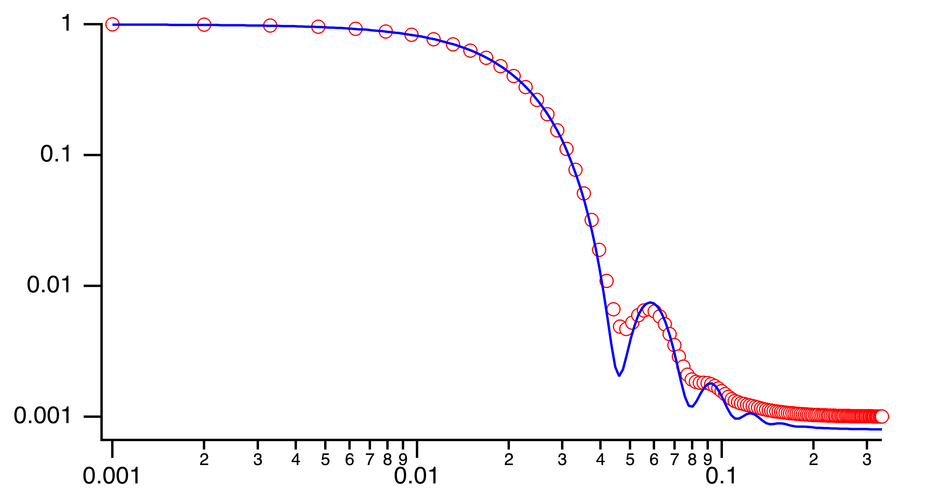
I have generated a model wave using the fit function (Plot_polyPq) and then tried to fit the model wave with the fit function (Fit_PolyPq).
The fit works but the convergence was poor and the errors of the coefficients were very large.
I have noticed there are many codes from NIST, but I need to build a much more complicated fit function for my actual data.
It will be great if you can give me some advice to improve this code.
#pragma TextEncoding = "UTF-8"
#pragma rtGlobals=3		// Use modern global access method and strict wave access.


Function Fit_polyPq(pw, yw, xw) : FitFunc
	wave pw, yw, xw

	variable scale, bkg
	variable Rc, sig

	scale = pw[0]
	Rc = pw[1]
	sig = pw[2]
	bkg = pw[3]

	wave pw2
	If(waveexists(pw2) == 0)
		make/o/n=3 pw2
	Endif
	pw2[0]=Rc
	pw2[1]=sig

	variable xmax, va, vb
	xmax = DimSize(xw, 0)
	va = -4*sig + Rc
	if (va<0)
		va=0		//to avoid numerical error when  va<0
	endif
	vb = 4*sig + Rc

	variable i
	For(i=0; i<xmax; i++)
		pw2[2] = xw[i]
		Yw[i] = Integrate1D(PolyPq_func, va, vb, 2, 0, pw2)
	Endfor

	Yw = scale*Yw + bkg

End


Function Plot_polyPq()

	make/o Yw, Xw
	Yw = 0
	Xw = 0.001 + 0.001*p^1.2

	variable scale, bkg
	variable Rc, sig

	make/o/n=4 pw = {1, 100, 10, 0.001}
	scale = pw[0]
	Rc = pw[1]
	sig = pw[2]
	bkg = pw[3]

	wave pw2
	If(waveexists(pw2) == 0)
		make/o/n=3 pw2
	Endif
	pw2[0]=Rc
	pw2[1]=sig

	variable xmax, va, vb
	xmax = DimSize(xw, 0)
	va = -4*sig + Rc
	if (va<0)
		va=0
	endif
	vb = 4*sig + Rc
	variable i
	For(i=0; i<xmax; i++)
		pw2[2] = Xw[i]
		Yw[i] = Integrate1D(PolyPq_func, va, vb, 2, 0, pw2)
	Endfor

	Yw = scale*Yw + bkg

	Display Yw vs Xw
	ModifyGraph log=1
	ModifyGraph mode=3,marker=8,opaque=1

End

Function PolyPq_func(pW2, inX)
	wave pw2
	variable inX

	variable avg, sig, qq
	avg = pw2[0]
	sig = pw2[1]
	qq = pw2[2]

	inX += 0.001

	variable gaus, pq, result

	gaus = (1/ ( sig*sqrt(2*Pi)) )*exp(-(inX-avg)^2/sig^2/2)

	Pq = 9*( sin(qq*inX) - qq*inX*cos(qq*inX))^2
	Pq /= (qq*inX)^6

	result = gaus * pq

	return result

End
I get a perfectly fine result with Igor 8 / 9 beta. Which version are you using?
By the way, I have adjusted the code to make it more readable (for me, to spot possible problems). This may have changed the result already. Just try this one and see what you get:
December 17, 2020 at 06:55 pm - Permalink
Thank you for your help. I am using Igor 8. The fit works if I set fit coefficients very close to those on model curves.
Otherwise, it fails.
I have set the initial guess as pw = {1.2, 120, 13, 0.008}. The expected coefficients should be pw = {1, 100, 10, 0.001}
December 17, 2020 at 08:29 pm - Permalink
I see. I did some further tests and find that the problematic parameters are the center R and sigma which translate into your integration range. Either the function gives some strange derivatives which makes it impossible for the fit to find the correct minimum, or there is just too heavy load and the fit gives up after a while. I don't know the details of the fitting functionality well enough here. My guess would be that sigma is the culprit, which controls both the integration range and the shape of your input function. This may lead to unexpected results and the fit has no idea how to proceed.
To improve things, could you reformulate your integration problem somehow? To at least speed up things (I hope), I would suggest to separate the integrant computation step and the integration itself. I think you can first compute PolyPq_func for all x (preferably using MatrixOp) and store the result in a (free) wave, and then integrate this wave later.
December 17, 2020 at 09:59 pm - Permalink
Have you considered evaluating the integral using FFT?
December 18, 2020 at 09:03 am - Permalink
This problem has been addressed in NIST code many times in one way (specific f(R)) and in Irena package other way (few different f(R)). I bet there are many other implementations in Igor, python,.. Polydipersed sphere is very basic example. I you want to talk to me directly (ilavsky@aps.anl.gov) we should be able to find solution. You could even use your own form factor in Irena Modeling tool - it enables user form factor and user structure factor.
Similarly to reflectivity, this is least-square nightmare case. Those Bessel function oscillations cause problems with fitting and if you are not close enough, you will never converge. With sufficient polydispersity this gets easier, but for close to monodispersed system like here, you must be close to converge in any case. Or you need to use something like Genetic Optimization which can find needle-in-haystack global solution.
December 19, 2020 at 01:38 pm - Permalink
In reply to I see. I did some further… by chozo
maru>chozo
Thank you for your advice. I have tried to reformulate the integration problem but could not find a good solution. Maybe, I did not really understand how to separate the integrant computation step and the integration itself in the Igor codes.
> igor
Can you give me an example to use FFT to evaluate the integral?
> ilavsky
I have checked the NIST codes, they have prepared a properly weighted 20-points-distribution to approximate the Gaussian distribution. The integration was performed by multiplying each point (different R) of the 20-points-distribution to P(q, R). This is a brilliant technique, but I wonder if there is a more versatile technique to perform the integration fits. I will directly contact you by email. Thank you for your help.
December 22, 2020 at 05:04 pm - Permalink