Get to Know a Feature: 3D Scatter Plots

Gizmo is Igor's 3D visualization tool.  It was completely revamped for Igor Pro 7.  In this blog post I'll demonstrate some variations of a scatter plot starting from the default scatter to an enhanced scatter plot.  

THE SIMPLE SCATTER PLOT

I'll start by generating sample data using makeSimpleLissajous(25). 

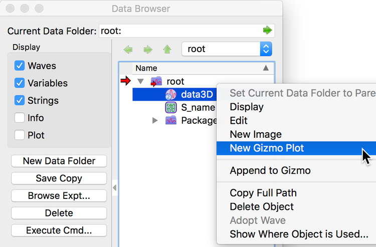
Next right-click the triplet wave data3D in the Data Browser and choose New Gizmo Plot.

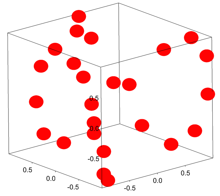
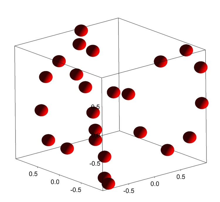
The default scatter plot and the associated Info window look like this:

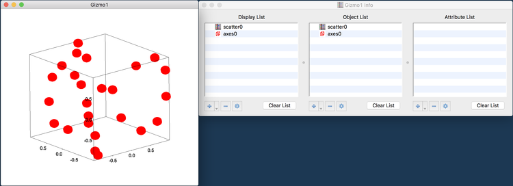
This is a basic representation of low-density 3D scatter which may be sufficient for some applications.  

ENHANCED SCATTER PLOT

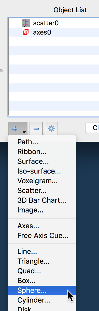
Since there are only 25 markers in the graph, each marker is large enough to justify additional computation to make it appear smoother.  To improve the default marker, create your own sphere object by clicking in the + icon at the bottom of the Info Window Object list and selecting Sphere... from the menu.

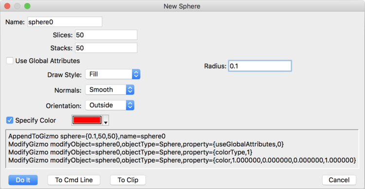
In the New Sphere dialog, change the number of slices and stacks to 50, the radius to 0.1, uncheck Use Global Attributes, and check Specify Color. Then click Do It.

Next you need to change the scatter marker to use the new sphere0 object that you just created.  To do so double click the scatter0 object in the Info Window and select Object from the Fixed Shape menu:

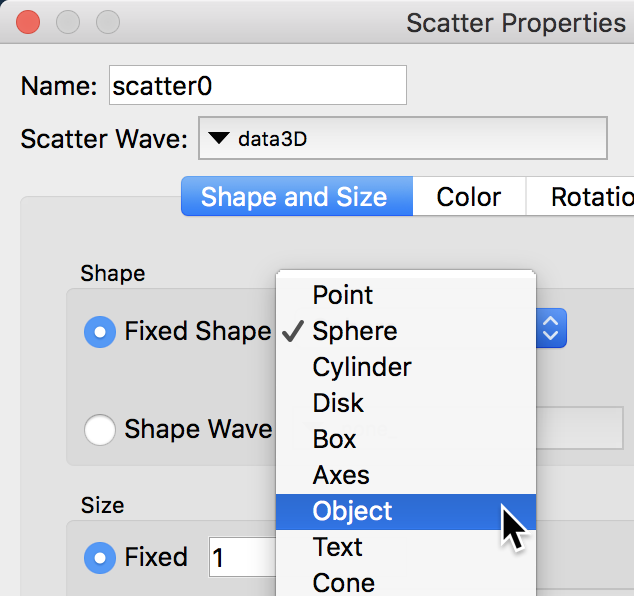
This will give you a second menu on the right from which you will choose sphere0 as your object.  The resulting graph has smoother spheres.

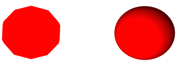
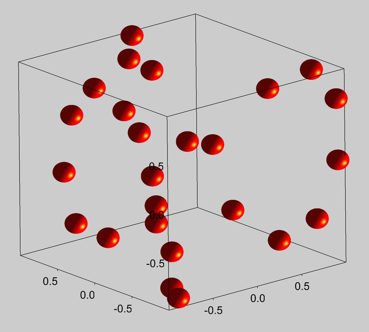
At this point it may be difficult to notice the difference between the default and custom spheres so I plotted side-by-side, magnified and added shading.  The default sphere on the left consists of 10 and 10 stacks.  The custom sphere on the right consists of 50 slices and 50 stacks.  The default sphere on the left does not include computed surface normals so it is not shaded.

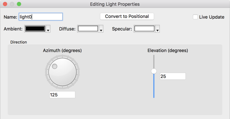
At this point you may decide that the scatter plot is sufficiently good but we are not going to stop here.  Instead add a light object to the Object List (click the + button and choose Light...) and in the Light Properties dialog set the Azimuth to 125 and the Elevation to 25 as shown below:

After you added light0 to the Info window, drag it from the Object List and drop it at the top of the Display List.

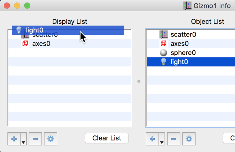
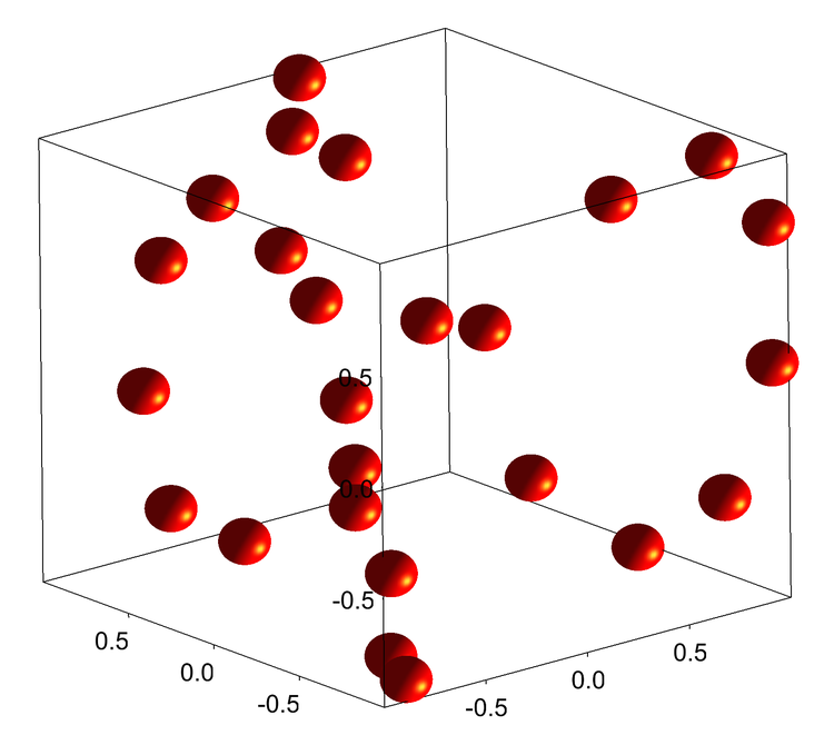
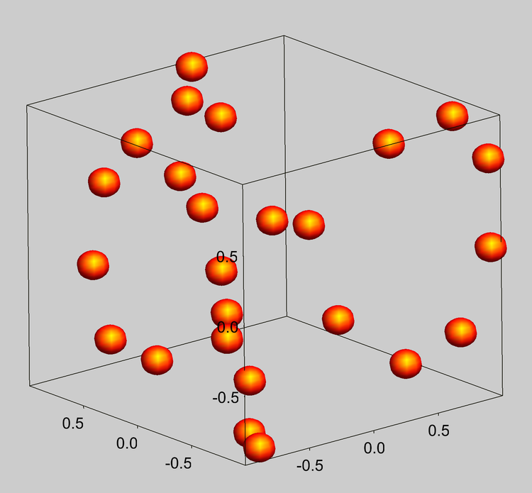
Your Gizmo plot should display the spherical markers with shadows similar to the graph below.

If you really want your spherical markers to stand out, you can add specular and shininess attributes.  You can do so by adding the items using the + button at the bottom of the Attribute List or executing the two commands:

Drag the two attributes from the Attribute List and drop them in the Display List above scatter0.  Your Display List should look like this:

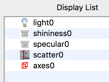
and your Gizmo plot should sport a specular reflection:

Depending on the medium you use to display your final result you may want add a final touch by changing the background color.  A simple gray background would look like this:

If you think that this is far too much work for generating one sparse 3D scatter plot you might appreciate the following command line shortcuts:

NewGizmo; appendtoGizmo defaultscatter=data3d
Modifygizmo enhance

These two lines of code generate the following graph.  It only differs from the one we created above in using low resolution default spherical markers.

In the next Gizmo post I'll focus on the path defined by the sequential scatter points.