How to compute and display scalp potentials from EEG recordings

Created on July 7 at 12:34 pm - by: admin

EEG researchers commonly create spatial maps of the electrical activity acros the scalp. Data are interpolated or triangulated from a discrete number of electrode placements distributed across the scalp (generally greater than 32 sites) often in fixed/standardized positions (see, e.g., http://www.ant-neuro.com/products/waveguard_original).

To do this, electrode coordinates, either as {x, y, z} triplets or in spherical coordinates are needed and can be obtained from the manufacturer of electrode caps (e.g., https://www.egi.com/knowledge-center/item/71-sensor-position-files-for-visualizing-data-in-third-party-software).

Theoretical analysis typically involves modeling the head as a perfect sphere. The mapping of the electrode coordinates to the surface of a sphere can be accomplished with the following function:

Function scaleToSpherical(inWave)

    Wave inWave

    // offset the coordinates to the  origin:

    MatrixOP/o/free wave0c=subtractMean(inWave,1)

    // compute the distance of electrodes from the origin:

    MatrixOP/O/free rawRad=sqrt(magsqr(col(wave0c,0))+magsqr(col(wave0c,1))+magsqr(col(wave0c,2)))

    // rescale the distance to a radius of 1:

    MatrixOP/O centeredNormalized=scalerows(wave0c,rec(rawRad))

End

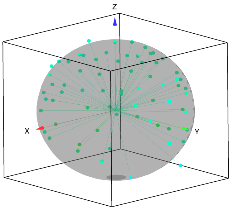
Figure 1: Initial electrode positions relative to the surface of a sphere.

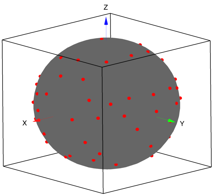
Figure 1:Initial electrode positions relative to the surface of a sphere.

Figure 2: Normalized electrode coordinates on the surface of a sphere.

Figure 2: Normalized electrode coordinates on the surface of a sphere.

Using the normalized set of coordinates we can triangulate the data on the surface of a sphere using the SphericalTriangulate operation.

SphericalTriangulate centeredNormalized // this creates M_TriangulationData

Following the triangulation we can use the wave M_TriangulationData combined with the EEG data to interpolate the potentials at any point on the sphere. In order to display the resulting interpolation in Gizmo we start by creating a parametric surface representing the sphere.

Function makeParametricSphere(pointsx,pointsy)

    Variable pointsx,pointsy

    Variable i,j,rad

    Make/O/N=(pointsx,pointsy,3) parametricW

    Variable anglePhi,angleTheta

    Variable dPhi,dTheta

    dPhi=2*pi/(pointsx-1)

    dTheta=pi/(pointsy-1)

    Variable xx,yy,zz

    Variable sig

    for(j=0;j<pointsy;j+=1)

        angleTheta=j*dTheta

        zz=sin(angleTheta)

        if(angleTheta>pi/2)

            sig=-1

        else

            sig=1

        endif

        for(i=0;i<pointsx;i+=1)

            anglePhi=i*dPhi

            xx=zz*cos(anglePhi)

            yy=zz*sin(anglePhi)

            parametricW[i][j][0]=xx

            parametricW[i][j][1]=yy

            parametricW[i][j][2]=sig*sqrt(1-xx*xx-yy*yy)

        endfor

    endfor

End

To complete the interpolation we need to construct one more wave: dataPointsWave. This wave has 4-columns consisting of the electrode coordinates in the first three columns and the potentials measured by each electrode at some fixed time t0 in the fourth column:

Variable nRows=DimSize(centeredNormalized,0)

    Make/O/D/N=(nRows,4) dataPointsWave

    dataPointsWave[][0,2]=centeredNormalized

    dataPointsWave[][3]=electrodePotentials[p]

The interpolation is computed by:

SphericalInterpolate M_TriangulationData,dataPointsWave,sphereData

The resulting interpolation is stored in the wave W_SphericalInterpolation where each row contains the scalar potential interpolated for the corresponding XYZ location in the wave sphereData. To display these values on the parametric surface we need to construct a color wave

Function createParametricColorWave(pWave,interpWave,reverseCTAB)

    Wave pWave,interpWave

    Variable reverseCTAB            // set to 1 to reverse; 0 otherwise

    // the color wave must match the parametric surface:

    Variable rows=dimsize(pwave,0)

    Variable cols=dimSize(pWave,1)

    // Create the parametric color wave:

    Make/O/N=(rows,cols,4) pWaveColor=1     

    // find the range of values for scaling:

    Variable mmax=WaveMax(interpWave)

    Variable mmin=WaveMin(interpWave)

    // optionally replace the colortable here:

    ColorTab2Wave rainbow256

    Wave M_Colors

    // not all colortables have the same number of colors:

    Variable nTableCols=DimSize(M_Colors,0)-1

    if(reverseCTAB)

        MatrixOP/o/free aa=col(M_Colors,0)

        WaveTransform/o flip aa

        MatrixOP/O M_Colors=setCol(M_Colors,0,aa)

        MatrixOP/o/free aa=col(M_Colors,1)

        WaveTransform/o flip aa

        MatrixOP/O M_Colors=setCol(M_Colors,1,aa)

        MatrixOP/o/free aa=col(M_Colors,2)

        WaveTransform/o flip aa

        MatrixOP/O M_Colors=setCol(M_Colors,2,aa)

    endif

    MatrixOP/O M_Colors=fp32(M_Colors/65535)

    Variable nor=nTableCols/(mmax-mmin)

    Variable i, np=rows*cols,index,rr,cc

    for(i=0;i<np;i+=1)

        index=trunc((interpWave[i]-mmin)*nor)

        rr=mod(i,rows)

        cc=trunc(i/rows)

        pWaveColor[rr][cc][0]=M_Colors[index][0]

        pWaveColor[rr][cc][1]=M_Colors[index][1]

        pWaveColor[rr][cc][2]=M_Colors[index][2]

    endfor

End

An example of this approach is illustrated in a cross-lingustic speech discrimination study at the following webpage:

http://www.gc.cuny.edu/Page-Elements/Academics-Research-Centers-Initiatives/Doctoral-Programs/Speech-Language-Hearing-Sciences/Research-Labs/Developmental-Neurolinguistics-Laboratory/Research-Highlights

Valerie L. Shafer, Ph.D.
vshafer@gc.cuny.edu
Professor and Deputy Executive Officer
Ph.D. Program in Speech-Language-Hearing Sciences
The Graduate Center, CUNY
365 Fifth Avenue, NY, NY 10016

Blog Posts Igor Pro 7

Forum

Support

Gallery

How to compute and display scalp potentials from EEG recordings

Igor Pro 9

Igor XOP Toolkit

Igor NIDAQ Tools MX