"Heat map" advice/opinion

Hello all,

I have a set of 2D coords and I'd like to plot the density of these points as a "heat map" (colour-coded map of probability at every location within a boundary). In the past, I have done one of two things:
1. 2D histogram - sample number of points in a grid and use that for representation, but this can look blocky. I have around 200 points so reducing bins can look weird with smaller bin sizes.
2. ImageInterpolate (voronoi) - for each point, calculate the number of neighbouring points within some arbitrary distance and use these values as z to make a surface with ImageInterpolate with voronoi option.

I'm wondering if a better approach would be to make a 2D gauss at each location and sum these together (perhaps with smoothing) to make the representation.
I'm not sure how to go about doing this other approach. I've tried to investigate the new StatsKDE option in IP7 without much success - does it work on 2D waves?

If anyone has:
- an opinion of what is the best way to make a heat map in these circumstances
- advice on how to do the third option.
I'd love to hear it. Otherwise, feel free to tell me to take this to stackexchange instead!
In IP7 you also have JointHistogram but that would not really get you over the fact that the small number of points would give rise to "blocky" output. If you take the result of JointHistogram you should be able to interpolate it directly (not using Voronoi because your result is already on a rectangular grid).

You might also want to check out the ImageFromXYZ operation.

FWIW: I think there is value in displaying the raw joint histogram results. The interpolation could lead you to misinterpret the results.
Thank you. I think you are right about interpolation being misleading. With so few points I can leave them as they are and set alpha at 0.5 or something so that overlapping points (as markers) appear darker.
sjr51 wrote:
Hello all,

I have a set of 2D coords and I'd like to plot the density of these points as a "heat map" (colour-coded map of probability at every location within a boundary). In the past, I have done one of two things:
1. 2D histogram - sample number of points in a grid and use that for representation, but this can look blocky. I have around 200 points so reducing bins can look weird with smaller bin sizes.
2. ImageInterpolate (voronoi) - for each point, calculate the number of neighbouring points within some arbitrary distance and use these values as z to make a surface with ImageInterpolate with voronoi option.

I'm wondering if a better approach would be to make a 2D gauss at each location and sum these together (perhaps with smoothing) to make the representation.
I'm not sure how to go about doing this other approach. I've tried to investigate the new StatsKDE option in IP7 without much success - does it work on 2D waves?

If anyone has:
- an opinion of what is the best way to make a heat map in these circumstances
- advice on how to do the third option.
I'd love to hear it. Otherwise, feel free to tell me to take this to stackexchange instead!


This is my code from years ago to do the third option you suggest. See here, for published example involving 2D maps of labeled neurons in brain sections
  • https://www.ncbi.nlm.nih.gov/pubmed/10376741

  • It assumes that x and y wave names are the same, except for ending with "x" and "y" respectively, and are generated from dataSetNameStr
    Xmin, Xmax, Ymin, Ymax are boundaries of the output image
    Pixelsize for output image is in whatever units your data are in, and Gaussian radius is the radius of the Gaussian kernel in pixels


    //******************************************************************************************************
    // Makes a 2D histogram with Gaussian smoothing
    Function TwoDHist_Gaussian (datasetnamestr, OutputFolderPath, Xmin, Xmax, Ymin, Ymax, pixelsize, GausRadius, DisplayNow)
        String datasetnamestr, OutputFolderPath
        variable Xmin, Xmax, Ymin, Ymax,  pixelsize, GausRadius, DisplayNow
       
        // make duplicates of the X and Y waves and trim them to Xmin, Xmax, Ymin, Ymax, plus a border equivalent to 3X the GausRadius
        // because cells that far away could affect pixels in the desired image space. Aterwards, we will crop the image.
        wave Xwave = $datasetnamestr + "x"
        wave Ywave = $datasetnamestr + "y"
        if (!(datafolderexists ("root:packages:twoDHist")))
            if (!(DataFolderExists ("root:packages")))
                newDataFolder root:packages
            endif
            newdatafolder root:packages:twoDHist
        endif
        duplicate/o Xwave root:packages:twoDHist:XWave
        duplicate/o Ywave root:packages:twoDHist:YWave
        Wave Xwave = root:packages:twoDHist:XWave
        Wave Ywave = root:packages:twoDHist:YWave
       
        sort  Xwave Xwave, Ywave
        // have to get rid of NaNs, they will be at the end after a sort
        variable ii
        For (ii = numpnts (Xwave) -1; numtype (Xwave [ii]) > 0; ii -= 1)
            Deletepoints ii, 1, Xwave, Ywave
        EndFor
       
        variable bs = BinarySearch(Xwave, xmin - (GausRadius * pixelsize * 3 ))
        if (bs > -1)
            DeletePoints 0, bs, Xwave, Ywave
        endif
        bs = BinarySearch(Xwave, Xmax + (GausRadius  * pixelsize * 3 ))
        if (bs > -1)
            DeletePoints bs, numpnts (Xwave), Xwave, Ywave
        endif

        sort Ywave Ywave, Xwave
        bs= BinarySearch(Ywave, ymin - (GausRadius  * pixelsize * 3))
        if (bs > -1)
            DeletePoints 0, bs, Xwave, Ywave
        endif
        bs= BinarySearch(Ywave, Ymax + (GausRadius * pixelsize  * 3))
        if (bs > -1)
            DeletePoints bs, numpnts (Ywave), Xwave, Ywave
        endif
       
        // Make a Gausian Blob of the required size.  After 3X the radius, the Gaussian function has fallen to about 3%, so we'll cut it off there
        // and make the blob size 6 times the radius, plus 1 for the center pixel. We'll also blank out the corners of the square image.
        variable GausPixWid = GausRadius * 6 + 1
        make/o/n = ((GausPixWid), (GausPixWid)) root:packages:twoDHist:GausBlob
        WAVE GausBlob = root:packages:twoDHist:GausBlob
        GausBlob = ((p - 3 * GausRadius)^2 + (q - 3 * GausRadius) ^2) <  (3 * GausRadius)^2 ? e^-(((p - 3 * GausRadius)^2 + (q - 3 * GausRadius)^2)/(2 * GausRadius^2)): 0
       
        // Make an  image bigger than we need, because of the margin of interaction issue
        variable xpixels = ceil((Xmax-Xmin)/pixelSize) + GausPixWid -1
        variable ypixels = ceil((Ymax-Ymin)/pixelSize) + GausPixWid -1
        make/o/n=((xpixels), (ypixels)), $OutputFolderPath
        Wave celim = $OutputFolderPath
        celim = 0
       
        //Now fill the image with the data
        // first transform the X,Y coordinates from mm into pixel space
        Xwave -= (Xmin  - (GausRadius  * pixelsize * 3)+ pixelsize/2)
        Ywave -= (Ymin  - (GausRadius  * pixelsize * 3) + pixelsize/2)
        Xwave /=PixelSize
        Ywave/=PixelSize
        variable numdata = numpnts (Xwave)
        For (ii = 0; ii < numdata; ii += 1)
            celim [max (0, (Xwave [ii] - (3 * GausRadius))), min (Xpixels-1, (Xwave [ii] +(3 *  GausRadius)))] [max (0, (Ywave [ii] - (3 * GausRadius))), min (Ypixels-1, (Ywave [ii] + (3 *GausRadius)))] +=  GausBlob [p - Xwave [ii] + (3 *GausRadius)] [q -Ywave [ii] + (3 *GausRadius)]
        endfor
        killwaves/z Xwave, Ywave, GausBlob      //  kill the temporary waves
       
        //delete the extra margins of the image
        DeletePoints /M=0  (xpixels - (3 *GausRadius)), (3 *GausRadius), celim
        DeletePoints /M=0  0, (3 * GausRadius), celim
        DeletePoints /M=1  (ypixels - (3 * GausRadius)), (3 *GausRadius), celim
        DeletePoints /M=1  0, (3 *GausRadius), celim
        SetScale/P x Xmin + PixelSize/2, PixelSize,"mm", celim
        SetScale/P y Ymin + PixelSize/2, PixelSize,"mm", celim
       
        // Display the image if so requested
        if (DisplayNow)
            display;appendimage celim
            ModifyGraph width={Plan,1,bottom,left}
            ModifyImage $nameofwave (celim) ctab= {*,*,Rainbow,1}
        endif
    end


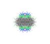
    I have attached a picture of some random data ovulated on its 2D gaussian blobbed equivalent

    make/n = 250 testx, testy
    •testx = enoise (5); testy = enoise (5) + 10
    •TwoDHist_Gaussian ("test", "root:OutPut", -6, 6, 3, 16, .05, 9, 1)
    append testy vs testx
    ModifyGraph mode=3,rgb=(0,0,0)

    Jamie Boyd, Ph.D.
    One additional thing you might want to do, depending on your needs, is to set the sum of the GaussianBlob to 1 after making it
    GausBlob = ((p - 3 * GausRadius)^2 + (q - 3 * GausRadius) ^2) <  (3 * GausRadius)^2 ? e^-(((p - 3 * GausRadius)^2 + (q - 3 * GausRadius)^2)/(2 * GausRadius^2)): 0 // after this line
    variable blobsum = sum(GausBlob)  //add this line
    GausBlob /= blobsum  // and this line

    so that the sum of the image will be equal to the number of points contributing to the image, for whatever size of kernel you use.


    Jamie Boyd, Ph.D.