Spectra Image Profile - Create profiles from, normalize and edit 2D / 3D spectral data

This project is used with 2D or (layers of) 3D data to create line profiles, and was inspired by the official Image Line Profile package (now replaced by the Line Profile function). The tool includes many convenient features tailored specifically to spectroscopic data (detector images, 2D scans or intensity maps etc.). Briefly, image data is integrated in horizontal or vertical direction within a region of interest (ROI, indicated by two lines). The resulting profile can be exported or used to modify the image data. Other features (such as normalization) are applied directly to the image data or layer. The tool modifies the input data directly, but a backup is saved upon start. Several convenient tools to work on 1D-3D data are included. The tool works directly on the input data, but a backup is saved upon start.
I tried my best to test everything thoroughly, but users should verify the correct behavior for critical applications. Bug reports and suggestions for new features are always welcome. Special thanks to Oleg Dyachok from Uppsala University for suggesting and testing improvements for version 4.0 and beyond.
User Interface (UI) controls
Select a 2D or 3D wave in the Data Browser and then go to ‘Spectra Tools’ → ‘Image Profile …’ in the main menu or use the command line:
SpectraProfile(inputWave)Below is an overview of all controls (here, the case of a 3D input is shown):
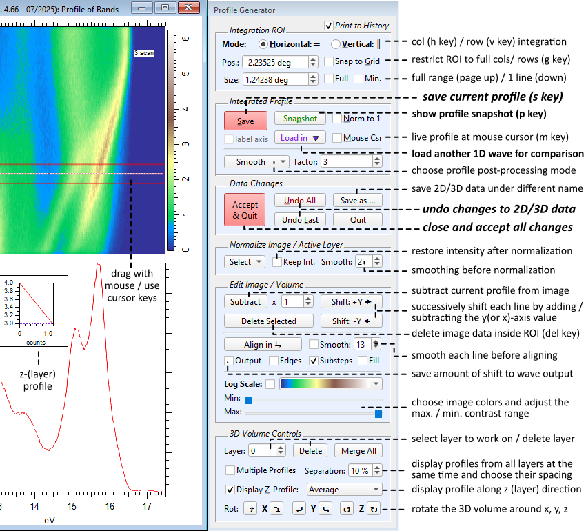
The tool prints a record of all actions to the history window. This can be switched off by unchecking Print to History.
Integration range (Region-of-Interest or ROI) controls
- The ROI lines can be dragged with the mouse directly with live updates of the profile. Dragging the (dashed) center line will move the whole ROI with the mouse. Dragging one of the (solid) side lines will stretch the ROI in the respective direction.
- While dragging the solid ROI lines: Hold the ctrl / cmd key to change the width symmetrically or hold the shift key to move the whole ROI (like when moving the center line).
- Choose the profile-integration mode: horizontal (h key) or vertical (v key) direction. Diagonal or free-form modes (like in the official Line Profile tool) are not available.
- ROI lines can be adjusted via the Pos. and Size values, by dragging the lines or by using the cursor keys on the keyboard.
- Right-click the Pos. / Size controls to load previous settings from compatible profile waves in the current folder (no menu will appear if no profiles are found).
- When using the cursor keys, hold the shift key to speed up changes by 4x. Hold the ctrl / cmd key to slows down changes by 1/2. Holding both the ctrl / cmd + shift keys slows changes down to one delta unit (one row / column).
- Snap to Grid: The ROI lines are constrained to include only full rows / columns.
- Switch to full or min. ROI range: activate the respective check box or use the page up / page down key, respectively.
Integrated Profile controls
- Norm to 1: The profile (not the image) will be normalized to fall between 0 and 1.
- Mouse Csr: An additional profile is plotted for comparison when the mouse cursor is moved across the image, which shows the current row or column under the mouse cursor (toggle with the m key). This profile is not saved.
- Save button: Saves the current profile in the folder of the input with a name-end tag depending on the selected range:
- The end tag is of the format “_H(xxx-xxx)” (horizontal mode) or “_V(xxx-xxx)” (vertical mode), where xxx is the start and end of the ROI range, e.g., “mydata_H(16.7-19.3)”. If the full image is selected the tag is “_prH” or “_prV”, respectively.
- Hold the shift key to force the use of “_prH” / “_prV” regardless of the selected range. The ROI position and size setting is always saved inside the output's wave note.
- Hold the alt key to save the output into the source wave's folder instead of the current folder.
- Activate the label axis checkbox to export additional axis information for plotting the output profile. This axis information is generated from the dimension labels of the source (if available) and exported as user-tick waves (with endings '_axV' and '_axT' for the axis value and label waves, respectively).
- Snapshot button: Creates and displays a backup of the current profile for comparison (this snapshot will not be saved). Each button press replaces this snapshot with the current profile. Hold ctrl to remove the current snapshot instead.
- Load in drop-down: Load an external wave (1D) for comparison with the current profile. This data can also be used for normalization (division), subtraction, and alignment.
- Profile post-processing options
Several options for post-processing applied to the profile are selectable via a drop-down menu. Post-processing will be applied live while the profile is changing, and is also saved in the output. It may be useful to apply post-processing before using other features such as division or subtraction. Available methods are: (simple) smoothing, Gaussian smoothing (via convolution), calculation of the integral and the derivative, and fast-Fourier transformation (FFT). FFT is not applied to the profile itself and is instead displayed in a subgraph. The FFT result is also exported using the end tag '_pp'.
Data Changes
- Accept & Quit: Closes the UI while keeping all edits made to the 2D/3D data so far.
- Undo All: Resets all changes made to the 2D/3D data (returns to the condition at start).
- Undo Last: Reverts the last change made to the 2D/3D data. This will only work once, i.e., you cannot undo multiple steps.
- Save as: Saves the 2D/3D data under a different name and undoes all edits made to the initial data.
- Quit: Closes the window undoes all edits made to the 2D/3D data.
Normalization
Normalization works only on the current layer of 3D data. The following normalization methods are available from the drop-down list:
- Divide by Profile: This divides the image / layer by the current or loaded profile (each column in horizontal / each row in vertical mode, respectively). Any selected profile post-processing is applied before this step, i.e., the profile as displayed in the main graph is used.
- Divide by Max. or Area: Finds the maximum or area of each row (horizontal mode) or column (vertical mode) and divides the column / row by this value. This is useful, for example, for equalizing data along one direction (use the Keep Int. checkbox to prevent downscaling of the data to 1).
- A user-defined function (this item is only displayed for compatible data): Normalize by user provided information. This can be any data parameter or wave saved in the current experiment. Examples are normalization by a secondary readout, time, concentration etc. See further below on how to set up your own normalization function.
Options:
- Smooth: The data / profile is smoothed before normalization is applied, which reduces the effects of noise in the input. Hold the ctrl / cmd key while selecting a normalization option to skip smoothing or set the value to 0.
- Keep Int. checkbox: This will preserve the average intensity after normalization, i.e., the data is scaled back to the initial, average intensity level.
The Delete Selected button
This deletes columns (horizontal) or rows (vertical) within the current ROI. If lines at the wave's edge are removed then the axis scaling is adjusted to account for the deleted lines. If lines in the center are removed then the scaling is not adjusted (wave scaling is linear and continuous and cannot account for missing points in-between). Be aware that this may break the relation between data and axis values. If the axis scaling is important (e.g., for a continuous energy scale), either refrain from using this feature or take care to only remove lines at the edges of the data. In case of 3D data, this feature will delete columns / rows on all layers.
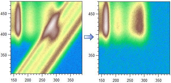
The Subtract button
The current (or loaded) profile is subtracted from each column (horizontal mode) or row (vertical mode) of the image / layer. This can be particularly useful for removing fixed spectral features across a scanned map. The scale (x) value can be adjusted to pre-scale the intensity of the profile before subtraction.
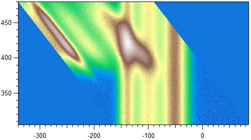
An additional function is available in horizontal mode only: the profile can be moved in x relative to the y-axis. Briefly, the y-axis value is added to (or subtracted from) the profile’s x scaling each step, which leads to a shifting profile in diagonal direction. This is useful to subtract features moving with increasing values on the y axis, such as peaks shifting with increasing photon energy.
- Hold ctrl / cmd to subtract while shifting towards increasing Y values.
- Hold alt / option to subtract while shifting towards decreasing Y values.
Below example shows a diagonal subtraction result (here using ctrl):
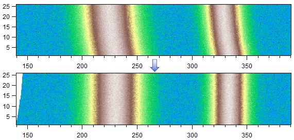
The Shift +/- buttons
Depending on the current mode, this tool shifts horizontal (vertical) image features: the x (y) value of each line is adjusted by adding (+) or subtracting (-) the increasing y (x) axis value of each line -> the resulting image is transformed into a parallelogram. All layers are processed for 3D. This tool will straighten features in the data which were shifting with y (x). An example would be a photon-energy scan of a spectrum where certain spectral features increase in their emission energy: Subtracting the photon-energy scale from a photoelectron spectrum in kinetic energy yields binding energy. The effect is illustrated again with above example data:
Hold ctrl / cmd to automatically delete any partially filled data after the shifting was done (the parallelogram is 'cut' down into a rectangle). Note that this is only done if there is enough of the data left after cutting (i.e., this is skipped if the parallelogram's skew is too large to fit a rectangle inside).
Align Features functionality
This tool searches for similar features in each column (horizontal mode) or row (vertical mode) of the image / layer and aims to align these features for maximum overlap by shifting each column / row by a certain amount. The algorithm uses wave correlation and shifts the data in whole steps (no interpolation) or, when the Sub-steps checkbox is active, sub-steps (interpolated). It is useful, for example, to correct slight shifts of peaks in a spectrum or to estimate the shift of a peak versus some other parameter like time or position:
The algorithm uses the first column (bottom to top in horizontal mode) or row (left to right in vertical mode) of the data as reference and tries to align all other columns / rows to this reference. Hold shift to use the last row / column instead (top to bottom in horizontal mode and right to left in vertical mode). If you want to align to the calculated or loaded profile instead, hold the alt / option key while pressing the Align Features button. A menu will appear which lets you select the desired reference.
Often, it is undesirable to use the full range of the data for alignment. By placing the A and/or B cursors onto the image you can limit the algorithm to the region between the cursors to, e.g., selectively align only a single feature of interest contained.
- Activate Smooth to smooth the data before aligning. This can improve the results for noisy data.
- Activate Edges to align for a maximum overlap of edge features instead of peak features (using the data's derivative).
- Substeps aligns in steps smaller than the data-point delta by using interpolation (default). Uncheck to shift in integer steps.
- Some data points will be outside the input range when shifting the data. Usually, these out-of-bounds data points remain unset (NaN). Activating Fill will instead repeat the end points of the data to fill this region.
- Activate Output to export found shift values into a wave with the name ending '_shft'. The image's wave scaling is applied.
Note that the algorithm is ‘dumb’ in the sense that it only looks for maximum correlation and does not judge whether 'peak features' really match etc. In the worst case this just aligns artifacts such as noise, so use with caution.
Image contrast and color controls
Here you can choose the used color table and adjust the contrast of the image / layer: select the desired color table by using the drop-down menu and move the Min and Max adjustment sliders until the contrast is as desired. The sliders are limited to the maximum and minimum data values of the image or current layer, so the contrast cannot be reduced only increased. If you reverse the Min / Max slider positions the colors of the image will be inverted. Activate Log Scale to switch to a logarithmic scale for both the image and profile. Switching to this mode will not work if the data is completely in the negative range or zero.
Additional controls for 3D data (volumes)
Layer and Merge controls
The Layer value selects the currently displayed layer of a 3D data set. Profiles are calculated from, and most functions for editing data will only act on, this one layer (there are exceptions like Delete Selection and Shift +/-). The Delete button deletes the current layer. The Merge All button will merge all (remaining) layers into a 2D image which can then be edited further. All changes can be reverted by using the Undo buttons. The scaled position of the current layer is shown as an annotation at the top right in the image.
Displaying profiles from all layers
Activating Multiple Profiles will simultaneously plot profiles of all layers, which are generated from the current ROI, for comparison with the profile of the current layer (shown in bold). The profiles will also be exported into a wave ending with '_map'. This is useful, e.g., to track small changes across many layers. The Separation value controls the vertical spacing between traces in the profile plot in percent of the (global) maximum y value. The maximum number of profiles (layers) which can be plotted is 200. Beyond this number the profiles are saved but are not shown.
Clicking Display Z-Profile will open an inset graph which plots the change of intensity in z- (i.e., layer-) direction, useful for tracking signal variations across layers. The type of information can be changed via the drop-down menu: average, maximum or minimum intensity.
Rotating a 3D volume
3D data can be rotated in 90-degree steps around the principal axes x,y,z in clockwise and counter-clockwise direction using the designated buttons at the bottom of the panel. After rotation the first layer is displayed by default, but if empty (zeros throughout) then the image might look all white (this is no bug). Rotation might reverse the x- and/or y-axes, depending on the new orientation of the volume's contents. Thus, the data might look 'reversed' when displayed in a normal image plot.
Quick-access functions in the menu
Some useful functions are available in the Spectra Tools menu and the right-click menu of the Data Browser:
- Append 1D,2D Datasets into 2D Data: Combines columns (y dimension) of multiple datasets into one consecutive 2D wave. The x dimension is extended to cover the full x range of all datasets if needed.
- Stack 2D Datasets into 3D Data: Stacks multiple 2D spectra (e.g., MCP images) to produce a 3D array.
- Profile of 2D\3D Data: Same as creating a profile over the full range using the UI. This will yield 1D data for a 2D input and 2D data or a 3D input. Hold shift while invoking this menu item to define a sub-range in the respective dimension.
- 2D Image from 3D Data: Sums 3D data in the layer (array) direction to output a 2D image.
- Split Up 2D\3D Data: Separates 2D / 3D data into individual waves holding columns, rows or layers, respectively. The individual waves are saved in a folder named after the input.
In Igor 9, these options are also available in the right-click menu of the data browser.
Creating profiles, splitting or combining data from the command line
Some quick access functions can be directly invoked. To create a profile use:
QProfile(input_wave, mode [,from ,to ,from_Point ,to_Point])Here the mode is an integer between 0 and 2, with the meaning of 0 = vertical profile (average rows), 1 = horizontal profile (average columns), 2 = z profile (average layers). Use the optional 'from', 'to' or the 'from_Point', 'to_Point' parameters to define the integration sub-range in terms of scaled values or point values, respectively. If both are specified the former takes precedence.
The data can be split along one dimension via:
QImageSplit(input_wave, dimension)Here, the dimension parameter has the same meaning as the mode above.
To reduce the fidelity of data you can bin data points by using:
QuickBinData(input_wave, binX, binY, binZ)Here, binX, binY, binZ must be integer values ≥1, which sets by how many points the data in the respective dimension is binned. For example, using binX = 2 will result in a wave with half of the points in the x (row) dimension (binning 2 points into 1). The input data can be binned in multiple dimensions simultaneously.
To combine data in the x- (rows), y- (column) or z- (layer) directions, use:
QuickCombineData(dimension, wave_list)The dimension parameter has the same meaning as above. wave_list is a string list of waves (use full paths if the waves are not in the current folder).
Procedure settings and user button code
The user-defined (normalization) button
Two functions and one global constant are used to provide the functionality for the user button:
- kUserInfoBtnName: Defines the menu item's description and can be dynamically changed to reflect the purpose of the function. This name should be short to fit inside the menu.
- Profile_ActivateUserInfoButton(inputWave): A function for deciding whether conditions for normalization are fulfilled. A return value of 1 activates, any other value disables user normalization. One could for example check here if the required information is contained in the 2D data or loaded in the current experiment.
- Profile_ExecuteUserInfoButton(inputWave): This function is called to do the normalization (or whatever you like to do here). Return a scaling factor for scaling the intensity to its average after normalization (returning 0 skips this step).
While this feature is intended for normalization, it is really a free-for-all function for any modification to the 2D data you may want. You could instead write a function which, for example, splits the data in half or applies interpolation or does something completely different in each experiment file.
You may modify the global constant and these two functions at the beginning of the procedure file directly, but it is more convenient to provide your own code in a separate file or inside the experiment environment. Use the Override keyword in front of the Function / StrConstant statement to override the standard definitions in your own implementation. You may use the project’s procedure code as basis for writing your own version. In the package, the function's purpose is to normalize to the ring current of synchrotron experiments as extracted from the 2D data as shown here:
static StrConstant kUserInfoBtnName = "Ring Current"	// the title of the user button

Static Function Profile_ActivateUserInfoButton(WAVE in)
	int activate
	// +++ conditions for activation +++
	activate = StringMatch(GetDimLabel(in,1,0),"*mA*")	// check if dim-labels contain "mA" values
	activate = StringMatch(note(in),"*ring current normalized*") ? 0 : activate	// already normalized?
	// +++
	return activate	// return 1 to activate button
End

static Function Profile_ExecuteUserInfoButton(WAVE in)
    variable valAvg = 0
    // +++ ring current normalization procedure +++
    variable value
    int dim = WaveDims(in); int i
    for (i = 0; i < DimSize(in,1); i++)
        string curLabel = GetDimLabel(in, 1, i)        // get the information from the column label
        sscanf curLabel, "%s (%f mA)", curLabel, value     // ring current info as "time (XXX mA)"
	if (value && !numtype(value))
	    if (dim == 3)
			in[][][i] /= value
	    else
			in[][i]   /= value
	    endif
        valAvg += value				// add the values for intensity re-normalization later
    endfor
    valAvg /= i+1
    Note in, "ring current normalized"	// write into note that the normalization has been done
    // +++
    return valAvg				// return the intensity normalization factor
End
Project Details
Current Project Release
| Release File: | Image Profile_v4.70.zip (46.26 KB) |
| Version: | IGOR.8.00.x-4.70 |
| Version Date: | |
| Version Major: | 4 |
| Version Patch Level: | 70 |
| OS Compatibility: | Windows Mac-Intel |
| Release Notes: |
|

Forum

Support

Gallery
Igor Pro 10
Learn More
Igor XOP Toolkit
Learn More
Igor NIDAQ Tools MX
Learn More
Wow. That single handily replaces 90% of the scripts I use every day with one convenient panel!
Thank you for sharing ?
February 18, 2021 at 02:19 am - Permalink
Great to hear. Thank you for your comment! I think this tool saves me the most time as well (others are graph-related tools which I haven't put up here yet ;). I guess the other 10 % are specialized scripts only related to your field? Please let me know if there is a feature which would make your (and others) life easier.
February 18, 2021 at 05:30 pm - Permalink
I couldn't help noticing the images for the Subtract Profile and Shift +/- sections. Those images look very similar to the Auger-yield NEXAFS data that we were battling with for a long time. In the end we used an iterative process to split up the data into vertical NECAFS and diagonal XPS contributions. If you are working with the same problems you might be interested in the paper.
"Removing photoemission features from Auger-yield NEXAFS spectra" https://doi.org/10.1016/j.elspec.2017.05.012
March 23, 2022 at 02:16 am - Permalink
Thank you for your comment and the link to the paper. I will take a look. Yes, this was exactly the reason for this functionality. The Subtract function relies on the fact that the XPS signal is present undisturbed in part of the scan and thus can be subtracted from the mixed image. We achieved this by simply measuring a sufficiently large range below the edge in question. This is of course complicated by second-order signal contributions, which are however often sufficiently small in our spectra. It might be interesting to add your approach to this package. What do you think?
March 23, 2022 at 04:38 am - Permalink
I did notice you expanded the kinetic energies far enough to where the Auger peaks are gone. I guess there are still some secondary electrons left, but it's good enough to where you can extract a reasonable XPS spectrum and subtract it.
If you want to try my approach out you can find it here www.wavemetrics.com/project/EccentricXPS
There is a pretty good help file and an example .pxp file you can test the cleanup procedure on. If you think it would fit into your package I would be happy to help you add it, but it's probably best if you test it first and see if you think it will fit.
March 23, 2022 at 10:57 am - Permalink
Load the examples file and run Photoemission Cleanup from the top menu
March 23, 2022 at 11:18 am - Permalink
My packages supports menu keyboard shortcuts which are loaded from a settings file. If you want to add keyboard shortcuts to common menu entries, place the content (Spectra Tools settings.dat) of the attached zip file in the same folder as the package procedure and edit as necessary.
July 27, 2023 at 11:55 pm - Permalink
This is great and thank you! Question, is it all possible to think about adding a Mode to visualize the 2D amplitudes across the layers in a 3D stack as they evolve with the Z-axis? Perhaps we could have it extract based on cursor location, or a specified Xmin-Xmax: Ymin-Ymax range that users change? I have data sets that display intensities over two frequencies (X & Y) that then evolve over time (Z). So, I have codes that extract that data automatically from specified ROI or from every single point in the 3D waves. But this generates large amounts of waves and graphs just to visualize the data trends. Igor also has good extraction tools, but to my knowledge this still requires extracting and plotting to visualize the data. Overall, images/maps are great for visualizing peak changes with frequency and/or time - no doubt. However, I spend a lot of time analyzing intensity changes at specific points, looking for rate differences, oscillations, FFT residuals, and then restacking said residuals into images.
Do you think adding a mode to visualize intensities plotted against the Z axis at specific X-Y coordinates is a feasible addition?! =)
November 8, 2023 at 01:42 pm - Permalink
Hi Electron, Thank you for your message and feature suggestion. This sounds quite interesting. I think it would be possible to show the evolution of intensity as a function of z at the mouse location and/or integrated overt the region of interest between the red lines. I don't think it will be that easy to show the intensity based on an user-chosen sub-region (like a marquee), since there is no code to handle marquees yet. Would a display at the mouse location enough for you? Would you want to know the integrated or 2D variation (z vs. x or z.vs. y, which would be a 2D image)?
November 8, 2023 at 09:48 pm - Permalink
In reply to Hi Electron, Thank you for… by chozo
Hi Chozo, thanks for your feedback. Displaying from the mouse location and/or integrated over a region would be very useful. I think showing the 2D variation over X or Y would be interesting additions. However, I initially had envisioned showing the intensity at the given point a specified 1D wave. I think even the option to just show the Z intensity against number of points (layers) as one moved the cursor around would be very helpful! I hope that makes sense, and I am happy to assist in anyway I can - although my programming skills are still young =).
November 9, 2023 at 08:32 am - Permalink
OK, attached is a start. You have to activate both 'Display z-Profile' and 'Mouse Profile' for now, since I have implemented only this one feature. Then you can move the mouse across any point to see the profile there. Regarding the integrated z-Profile, I am still unsure how to display this information, i.e., either as (fake) waterfall plot or image. What do you think?
November 9, 2023 at 06:43 pm - Permalink
Nevermind, it was not so difficult to add a function to integrate the ROI in both x- and y- to create a z profile. Please try out the attached procedure and let me know if that is what you have envisioned.
November 9, 2023 at 10:09 pm - Permalink
In reply to Nevermind, it was not so… by chozo
This works well - much obliged. Scanning the cursor around to visualize z-profiles is seamless and prevents me from generating large amounts of waves. Thanks!
November 10, 2023 at 08:09 am - Permalink
@Electron: I have now added this feature into the official version, although in a slightly different way as in the test version.
December 7, 2023 at 01:10 am - Permalink
In reply to @Electron: I have now added… by chozo
Thanks, Chozo - much appreciated.
December 7, 2023 at 08:04 am - Permalink
Hi! This is a great code for spectra image analysis, many thanks! I have quite a silly question since I am trying to plot the peak shift vs energy for some of my data. The 2D data I have does not contain the energy scale and I typically make the image plot for my 2D data vs energy (1D wave). However, in the image profile of the Spectra tools kit, it only plots the 2D wave, thus I am wondering if there is a way to be able to choose the x scale of the plot so that the peak shift will correspond to energy shift...
February 6, 2024 at 12:41 am - Permalink
Great to hear that you like the package! The support of scale-waves is on my long term feature list, but it turns out this interferes with the (red) profile lines especially for non-linear x waves.
I am not sure I understand fully what you are trying to do. What do you mean by "peak shift"? Is this about the output of the 'Align' feature? You could simply use the output and plot it versus your 1D wave for scaling. I think you would need to recalculate the scale a bit, since x waves for 1D and 2D data works a bit differently.
Would it be possible to attach some example data here? Then I can guide you through the process.
February 6, 2024 at 12:35 pm - Permalink
I appoligize, it might be confusing and hopefully will be more clear with some data. I try to send in here a 2D data (spectra as a function of time) and 1 D data (energy scale) as an example. I am interested into plotting the peak position in energy (or shift) as a function of time for the different spectra recorded. As for now the output of the 'Align' feature gives me some shift (in some numbers which are not connected to energy) vs time. I would like the y-axis to be energy of some kind. Hope that this became a bit more clear. Thank you!
February 7, 2024 at 12:53 am - Permalink
No need to apologize. I see what you want to try clearly know. First note that the Align feature compares and shifts whole rows (unless you specify a limited range via cursors). The output is in data points, i.e., how many points each row has been shifted over to match. So you would need to multiply these number with the energy delta, i.e., how much energy each point corresponds to. Looking at your energy scale, there is quite some fluctuation; the step between each energy is not constant. What you can do is to assign an 'average' energy delta to the output. This is the same as applying a linear scale to your image before using my Image Tool. Here is how you can do that. Execute the following for your example data:
The last factor is basically the average energy step calculated from energy_scale.
If you want to properly take the variable energy spacing into account then you would need to first interpolate your 2D_wave into a linear scale. You could use interp2D for that, but it is a bit more involved. Then you use my Image Tool on the transformed data. Since your energy-step fluctuations are quite small compared to the rather large shift you observe, the result would not be that affected (i.e., the error you get with above simple approach is small). Let me know if you are interested and I can walk you through that as well.
February 7, 2024 at 02:20 am - Permalink
Many thanks, Chozo! This seems to work pretty well now so it is already good for my data! Since I have plenty of data with even smaller energy shift it might be worth looking into the linear scale interpolation of the image if it is not too much to ask for (just to make sure I don't miss any shifts?). Will it be somehow possible to obtain the energy position (instead of shift) of the peak vs time?
February 7, 2024 at 06:40 am - Permalink
The Align feature does not know anything about your data, it's shape, position etc. So it is impossible to define a 'position' automatically for arbitrary data. You can do the following, however: Find out the peak position at the beginning yourself and then just add the energy shift to that value. I fitted the larger peak at the very bottom of your 2D image and got 96.976 points for the start position, which is:
Now you can do:
This gives you the position for that 'peak'. Note that the shape is not well defined at the beginning of 2D_wave. You could also use some position which is well defined at the center of the data and work from there. Just make sure you find the correct offset. Note that you can also use the Align feature in reverse: Hold 'shift' to align to the top row as reference. This might be better if the bottom rows are noisy or have some other issue. Maybe at some point in the future I offer to align to an arbitrary reference.
I will get back to you regarding the interpolation later.
February 7, 2024 at 02:22 pm - Permalink
In reply to The Align feature does not… by chozo
Thank you very much, Chozo for all your help! This really saved me some time! I have checked now some other data with smaller shifts and I think the approach you suggested works well enough for my data. So don't bother about the interpolation, this is already very good and I am very thankful.
February 8, 2024 at 07:07 am - Permalink
Great to hear that. Just let me know when the interpolation might become necessary or you have any other requests.
February 8, 2024 at 07:59 am - Permalink