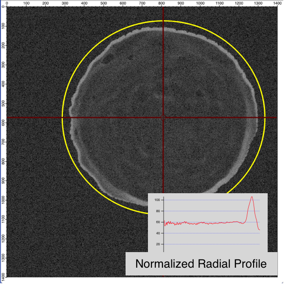
Radial Profiler

This code will generate a radial profile across a circular region in an image. It follows on the starting point posted here: https://www.wavemetrics.com/node/20946
// create a radial profile in an image
// simg - 2D image wave
// cx, cy - center for circle in image
// rmax - maximum radius to take profile
// creates profile waves: M_RadialProfile, M_RadialProfileWeights, M_NormRadialProfile
// creates variables: V_TotalArea, V_TotalIntensity

Function CreateRadialProfile(simg, cx, cy, rmax)
	wave simg
	variable cx, cy, rmax

	variable ix, iy, ixmax, iymax, rpos, rposf, rposc, pmax

	Make/D/O/N=(rmax+1) M_RadialProfile=0, M_RadialProfileWeights=0, M_NormRadialProfile=0
	variable/G V_TotalArea, V_TotalIntensity
	V_TotalArea = 0; V_TotalIntensity = 0

   ixmax = rmax
   // outer sum over x
	for (ix=1-ixmax; ix<ixmax; ix+=1)
		// bound y by current x
		iymax = floor(sqrt(rmax^2 - ix^2))
		// inner sum over y
		for (iy=1-iymax; iy<iymax; iy+=1)
			rpos = sqrt(ix^2 + iy^2)
			// split value between the two closest points in the radial profile wave
			rposf = floor(rpos)
			rposc = ceil(rpos)
			// fill the weighting array
			M_RadialProfileWeights[rposf]+=(rpos-rposf)
			M_RadialProfileWeights[rposc]+=(rposc-rpos)
			// fill the profile array
            M_RadialProfile[rposf] += simg[cx+ix][cy+iy]*(rpos-rposf)
            M_RadialProfile[rposc] += simg[cx+ix][cy+iy]*(rposc-rpos)
            // add to the total area and total intensity
            V_TotalArea += 1
            V_TotalIntensity += simg[cx+ix][cy+iy]
		endfor
	endfor
	// generate normalize profile
	M_NormRadialProfile = M_RadialProfile/M_RadialProfileWeights

	return 0
end
A few further thoughts:
* I have to wonder whether some of this code could be multithreaded.
* When you want to generate a radial profile but exclude certain parts of the image that are within the circle (e.g. take a radial profile but only over half the circle), set those parts of simg to zero that you want to exclude.
* An alternative method to obtain a radial profile is to step through using ImageLineProfile with circular profiles as mentioned in this post https://www.wavemetrics.com/forum/general/radial-profiles-sector-integration . This latter method would lend itself more readily to creating ellipses or doing other tweaks (e.g. using the profile width as a way to average radially). I would be curious about the differences in accuracy and speed of the two approaches (brute force pixel-by-pixel conversion versus radial-line-profile averaging).
Finally, I would like to see this function become a built-in operation in Igor Pro (e.g. ImageRadialProfile/C={cx,cy}/R={rmax} simg).

Forum

Support

Gallery
Igor Pro 10
Learn More
Igor XOP Toolkit
Learn More
Igor NIDAQ Tools MX
Learn More
I'm not sure what you are trying to accomplish with this code that is not done in ImageLineProfile. It seems to me that this function may give you results that are similar to ImageLineProfile with width=0 but without the interpolation. If you use width>0, ImageLineProfile can also provide you with some stats for every sample point on the variation of the data in a direction perpendicular to the path. Another incentive to use ImageLineProfile is that it is automatically multithreaded.
I don't know how to answer your question regarding accuracy. For example, in some applications you may consider a bilinear interpolation to be inaccurate so it would be helpful if you defined your requirements. Also, ImageLineProfile may oversample your domain relative to your code.
A.G.
January 28, 2020 at 12:04 pm - Permalink
AG:
Perhaps the better statement than saying that I believe the pixel-by-pixel method to be accurate for analysis *on any one image* (e.g. versus some other method) may be to say that I trust the pixel-by-pixel method to be robust in principle and accurate in practice when it is used for *comparative* analysis of results from one image versus another.
As time permits, I hope to explore the differences in results between the pixel-by-pixel scan method and ImageLineProfile with a radially defined wave profile. I am certainly intrigued by what might be learned in a side-by-side comparison of results for pixel-by-pixel versus ImageLineProfile using a width=0 as well as in the statistics from ImageLineProfile using a width>0. I am also enticed by the possibility to generate profiles using elliptical or other coordinates as well as to do only partial profiles in angular coordinates.
Thanks!
January 29, 2020 at 06:41 am - Permalink
It seems to me that methods that avoid interpolation cannot be applied to anything but straight (horizontal or vertical) lines. otherwise you have a tradeoff between interpolating values (bilinear) or deviating from the true mathematical path (Bresenham). In a way, one can look at this as analogous to trying to draw a nice round circle on a binary image.
I would be interested in any insights you might have on ImageLineProfile.
AG
January 29, 2020 at 05:51 pm - Permalink
Here is an updated version.
* Method = 1 - Pixel by Pixel with Linear Interpolation
* Method = 2 - Pixel by Pixel with Quadratic Interpolation
* Method = 3 - Radial Wave Profile with ImageLineProfile
Notes
* The three methods give comparable (nearly identical) results for the M_RadialFluxProfile result. I have not clocked the methods for time comparisons.
* In Method 3, I use of value r360 to calculate the radius where the circular profile would have 360 points at an angular resolution of 1o. I scale the resolution of the radial profile down with r < r360 and up as r > r360.
* Method 3 affords the greatest options for future expansion, including coding for a) variable angular resolution, b) limiting angular slices to defined start and end angles (pie slices), and c) using profile widths > 1 to obtain statistics from ImageLineProfile.
* In Method 3, I do not pay any attention to scalings on the source image. So, if your image has x, y scalings and you do not care to figure out how to remove them BEFORE the method, you are better to use the "brute force" pixel-by-pixel method.
I have already built the above code for a radial profiler into a control panel. It works in conjunction with the Image Tools package. I would be glad to provide a release to anyone who might want to test it.
February 10, 2020 at 12:04 pm - Permalink
When you get access to IP9 look for ImageLineProfile with the /RAD flag.
A.G.
February 13, 2020 at 12:03 pm - Permalink
In reply to When you get access to IP9… by Igor
Pray tell when will that be?
Andy
February 13, 2020 at 12:18 pm - Permalink
I was going to say "real soon now"...
Are you also interested in this feature or just interested in the timing for IP9 beta?
February 13, 2020 at 12:27 pm - Permalink
Both actually.
I have written a couple of applications for clients doing either doing radial profiling explicitly or have used it behind the scenes for other algorithmic purposes. ImageLineProfile is a very nice function.
Andy
February 13, 2020 at 01:06 pm - Permalink
AG: I am glad that my effort inspired the addition to Igor Pro 9. From a user standpoint, the amount of time I had to invest to figure out the details on my own should not be something that future users should have to repeat. I would have wanted and still wish for a single line command to * carry out radial profile analysis * + * starting centered at this position * + * going out this far * + * using this angular resolution * + * over this angular range* + * applying this line width *.
So, with this in mind and when it is not too late, I would (again) petition for a dedicated command with inputs along this line:
C = (x,y) center position in scaled coordinates
C = [px, py] center position in point coordinates
-- default in both cases is center of image
THETA=(start, end) start to end range of angular sweep in degrees, default is (0,360)
RMAX=(value) maximum radius to extend using coordinates set by C
- default is points extending until the first boundary met in the image (i.e. minimum of (width/2 - cx) or (height/2 - cy)
RES=(value) angular resolution factor for points in each radial profile determined as npts = 2*Pi*r/RESAndy and others: Let me know off-line when you would like have access to the add-in panel code to Image Tools that will do radial profiling. I cannot foresee anytime soon enough when the panel code will become a plug-in to Image Tools, and I am likely not to release the panel code as a stand-alone package to IgorExchange.
Andy and Others: The radial profile panel works robustly as a stand-alone package in parallel with Image Tools. I am inclined at this point to post it only to those in need. Contact me off-line.
February 14, 2020 at 09:52 am - Permalink
The IP9 implementation is a bit more complicated allowing for a default differential angle and when the width>0 it also computes the integrated intensity for the annular domain.
February 14, 2020 at 04:38 pm - Permalink