Parallel coordinate plot with smooth lines?


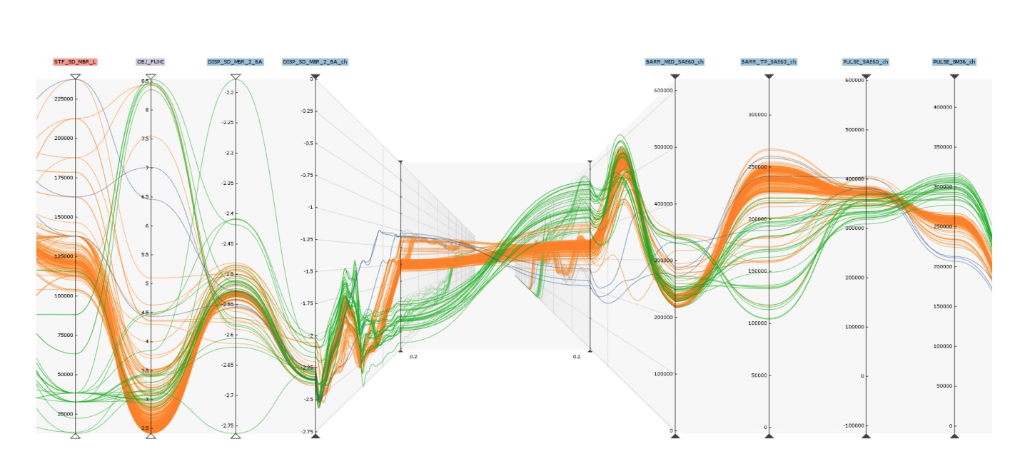
I have always found Parallel coordinate plots (https://en.wikipedia.org/wiki/Parallel_coordinates) bit difficult to read and enough confusing not to use them. Recently I saw the same plot with smooth curves instead of straight lines and found it surprisingly better for human eye. See attached figure.
I would like to find way to generate these from my results in Igor. I am running into some issues creating the smooth curves connecting the data points. I tried playing with Interpolate2 cubic spline, but it is not resulting in what I need. It does not guarantee that derivative of the curve in each point (crossing each vertical line) is 0 so it generates curves which have maxima and minima away from the data points / lines. See maximum on spline curve in my plot around 2.3 and minimum around 3.8.
Wikipedia even has link to paper which discusses what needs to be satisfied to make these lines look as expected. Reference 7 on https://en.wikipedia.org/wiki/Parallel_coordinates
Anyone has suggestion how to generate these spline curves in Igor?
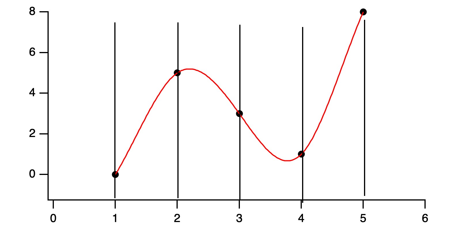
Does it work to use two points at each maximum/minimum, one slightly on each side of the intended vertical line? That is, two points with the same Y value, and X values at x0-dx and x0+dx. It seems like that should force a zero derivative through those two points, though splines can do some weird things. I suppose you might even have to add a third point at x0 to really force the derivative to zero.
March 16, 2021 at 10:00 am - Permalink
In reply to Does it work to use two… by johnweeks
KurtBPerhaps the smoothed curve could be constructed using a cosine function (0 to pi) with an appropriate vertical and horizontal scaling factors, and with one half-period between each set of points?
March 16, 2021 at 10:18 am - Permalink
set the first derivative to zero and match the second derivative of connecting segments at the nodes - I guess that's just a restatement of the problem.
the cubics then look something like this:
y = y0 + 3(y1-y0)*t^2 + 2(y0-y1)*t^3
where t = (x-x0)/(x1-x0), nodes are x0,y0 and x1,y1
(I scribbled this down on a piece of paper, and didn't check to see if it's right).
Someone else can supply the neat linear algebra solution.
EDIT: I checked this against the curves in the image, and while it satisfies the zero gradient and matching second derivatives, it doesn't have quite the same shape as the curves on the plot. Should have read the reference, I guess. It does look the same as the cubic spline solution below, though. It would be worrying if it didn't!
March 16, 2021 at 10:24 am - Permalink
In reply to Does it work to use two… by johnweeks
ilavskyI added to each node a point 0.01 before and 0.01 after its x value with same Y value and I got what I needed. This is easy solution.
I really want to use some fast Igor function since this will be done for many curves at once so speed is important also. These graphs can get messy...
Thank you, this was easy.
March 16, 2021 at 11:00 am - Permalink
Now- what does that plot mean?
March 16, 2021 at 12:42 pm - Permalink
In reply to Now- what does that plot… by johnweeks
ilavskyThe one I made? Nothing. But normally Parallel coordinate plot can be useful for visualization of large sets of data where you can easier identify trends. One can visualize what groups of data have similar some parameters. If I have system with input parameters A, B, and C which yields measured/modeled values Z, X, Y, it is difficult to present all A, B, C, Z, X, Y in one graphics and still make some sense. This is one way to do it.
Typically one would have some number of input parameters (some number of left vertical axes) and then some output parameters (other vertical axes). Each line represents one measurement and connects all input and output values. One can visualize quickly which parameters yield similar results. Or which output results are related to which input values. Typically this plot uses straight lines but this one is somehow easier to understand and follow.
The trick is to add tools for user to help - for example way to select some lines with similar parameter on one axes and color them to see, what other parameters look like or what are common input parameters.
March 16, 2021 at 02:05 pm - Permalink