Super Quick Fit - Quick Fit with more options, derived values output and user-function support
This project replaces the built-in Quick Fit. Super Quick Fit covers every function of Quick Fit and adds several convenient features. Right-click on a graph or trace to invoke the menu.
Special thanks to Oleg Dyachok from Uppsala University for suggesting and testing improvements for version 1.05 and beyond.
I tried my best to test everything thoroughly, but sometimes bugs slip through. Bug reports and suggestions for new features are always welcome. I am happy to add more useful settings, peak shapes or derived values if I receive feedback. Currently, 2D fit support may not be perfect since I don't have any meaningful data to test everything. If you have suggestions for improvement of 2D fitting or can test this functionality in detail, then please let me know.
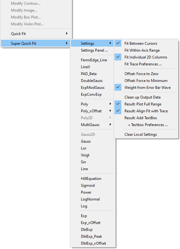
More settings:
- Fit Between Cursors - Same as for Quick Fit. Fit is limited to the range between cursors.
- Fit Within Axis Range - The fit range is limited to the top / bottom (and for images left / right) axis scale of the graph.
- Fit Individual 2D Columns - If the graph contains traces from a 2D wave, then each fitted column gets its own output wave named with the prefix 'fit_XX_'. XX designates the fitted column where the number of digits depends on the y-size of the wave (e.g., a wave with 200 columns would give 'fit_000_wavename' as output for the first column).
- Fit Trace Preferences - Opens a panel to choose the preferred fit-trace style (see below)
- Offset: Force to Zero - The 'offset value' of the fit function (most often the baseline value y0) is held at zero.
- Offset: Force to Minimum - The 'offset value' held at a minimum. The minimum is either determined by the minimum value from placed cursors or the minimum of the data (depending on the fit function this could be either a x or y minimum).
- Weight from Error Bar Wave - Same as for Quick Fit. The weight wave is taken from the error-bar wave of the trace.
- Clean up Output Data - Deletes output waves (other than the 'fit_' wave), strings and variables after the fit. Use this if you are only interested in the history output / the graph's text box and want to avoid accumulating W_coef, W_sigma waves etc.
- Result: Plot Full Range - Generate the output over the full axis range of the graph.
- Result: Align Fit with Trace - Scale and offset the fit trace in the same way as the source (i.e., align the fit to the source).
- Result: Add TextBox - Same as for Quick Fit. Adds a standard text box with result values to the graph.
- Textbox Preferences - Same as for Quick Fit. Choose what you would like to have printed into the result textbox.
Settings are saved in the current experiment (as root:QuickFitMenu_settings) to keep used settings consistent for each experiment file. Last-used settings are also persistent across Igor sessions, which makes it possible to set up your favorite work style as a default. Press Clear Local Settings to remove any settings of the current experiment (i.e., QuickFitMenu_settings) and load the persistent global settings instead.
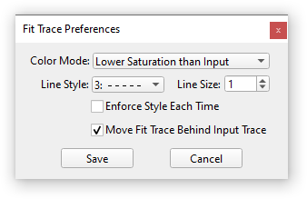
Fit Trace Preferences lets you set a preferred color and line style for new fit traces. This helps to make fit traces more distinct from the source trace. Already present fit traces are not affected unless you activate Enforce Style Each Time.
Additional Fit Functions:
(functions other than EMG are usable in the Curve-Fit dialog)
- FermiEdge_Line - Fermi–Dirac distribution combined with a linear slope.
Equation: f(E) = y0 + (m*E+A) / (exp((E-Ef)/kT)+1) - LineX - A line fit with the x-intercept (x0) as direct coefficient. Useful to determine x-intercepts with a low uncertainty, especially for lines with a steep slope. The default Line fit is based on y intercepts and not good at finding x-intercepts.
Equation: f(x) = m*(x-x0) - PAD_Beta - Angular distribution function, e.g., for analyzing photoemission experiments.
Equation: f(theta) = Scale*(1+Beta*legendreA(2,0,cos((theta-theta_0)*(Pi/180)))) - DoubleGauss - Two Gaussians combined to fit doublets. Does not work well for inputs without two clear 'peak' features.
Equation: f(x) = y0 + Area1 * Gauss(x,Loc1,Width1) + Area2 * Gauss(x,Loc2,Width2) - MultiGauss - A combination of up to ten Gaussians. Choose the number of functions from the menu. However, it is not guaranteed that the automatic guessing of peak parameters will be successful for the chosen number.
- ExpModGauss - Exponentially Modified Gaussian (EMG) peak shape. Equal to the one offered in the Multipeak Fit package.
- ExpConvExp - Convolution of two exponential decay functions. Equal to the one offered in the Multipeak Fit package.
- Use_Wave_Data - Fit a scaled and shifted source wave.
Output of Derived Values:
Additional derived parameters such as FWHM, area, height etc. (where applicable) are printed in history and the graph's text box. Currently, the following functions output derived parameters: LineX, DoubleGauss, MultiGauss, ExpModGauss, ExpConvExp, Line, Gauss, Lor(entz), and Voigt. You can also set up your own function to output additional derived values after a fit (see below).
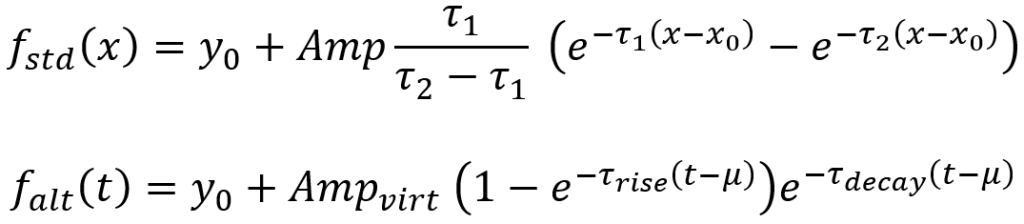
Alternative Derived Parameters for ExpConvExp:
The ExpConvExp function uses the standard functional form of the Multipeak Fit package, but derived parameters (virtual amplitude, inverse of the rise time, inverse of the decay time) for an alternative functional form are given at the same time. The alternative form is more common in some fields such as cell biology. Both functional forms are compared below:
Calling Super Quick Fit from the Command Line or Your Own Code:
Super Quick Fit can also be run in code by executing:
SuperQuickFit(string graphName, string traceName, string fitFuncName)'graphName' can be the name of any open graph or just "" for the top graph. 'traceName' can also be left empty ("") to fit an image plot or the first trace of the graph. 'fitFuncName' must be a valid built-in or user function name. SuperQuickFit() returns error codes (0 if the fit was successful). The last Fit settings are used and cannot be changed from code at present. Set up everything in the right-click menu first before running this function. It is most useful to fit multiple traces in a single graph or traces in multiple graphs.
The error codes are (if you use, e.g., print with the function call):
-1 = no valid target or function
-2 = no graph found
-3 = designated graph does not exist
-4 = trace not on graph
-5 = invalid function type
-6 = invalid contour trace
-10 = guess for fit function failed
-100 = image has separate x or y axis (not supported yet)
-999 = execution of the fit failed
Adding Your Own Fit Function:
Adding such functions is easy. Write a normal (such as created with the curve-fit dialog) or all-at-once fit function, then add a second one for calculating initial guesses. Let's look at a simple example, such as the LineX function included in the package:
function LineX(WAVE w, Variable x) : FitFunc
	//CurveFitDialog/ Equation:
	//CurveFitDialog/ f(x) = m*(x-x0)
	//CurveFitDialog/ End of Equation
	//CurveFitDialog/ Independent Variables 1
	//CurveFitDialog/ x
	//CurveFitDialog/ Coefficients 2
	//CurveFitDialog/ w[0] = x0
	//CurveFitDialog/ w[1] = m
	return w[1]*(x-w[0])
end
To calculate initial guesses (and to make this function appear as an item in the Super Quick Fit menu), you have to provide a function named YourFitFuncName+"_prepareCoef" with the SuperQuickFitStruct structure as input. In our example, the function must thus be named LineX_prepareCoef:
function LineX_prepareCoef(STRUCT SuperQuickFitStruct &s)
	Make/D/O/N=2 W_coef = {0,1}
	WAVE s.cw = W_coef
	return 0
end
The function must create a coefficient wave with the correct number of coefficients (two are needed for LineX) and fill initial guesses which are likely to make the fit succeed. The created coefficient wave then needs to be fed into the wave assignment s.cw. By the way, you don't have to call this wave W_coef. But if you choose this standard name, the coefficient wave will be properly deleted if you have the 'clean-up' setting active. Now you can select your function in Super Quick Fit.
In above example, the initial guesses are simply set to x0 = 0 and m = 1. This may be too simple for a good guess. You could also access the input data to calculate more reasonable guesses. The full function for LineX looks like this:
function LineX_prepareCoef(STRUCT SuperQuickFitStruct &s)
	WAVE temp_yw = SQF_getTraceWave(s)			// extract relevant trace data
	WaveStats/Q temp_yw
	variable Wmax = V_max					// get data's min and max value
	variable Wmin = V_min
	Differentiate temp_yw/D=temp_yw
	WaveStats/Q temp_yw
	variable slope = ((Wmax-Wmin)>0) ? V_max : V_min		// calculate slope from derivative

	Make/D/O/N=2 W_coef = {(s.holdMode==1 ? 0 : s.xBase),slope}	// prepare coefficient wave (2 points)
	WAVE s.cw = W_coef
	return 0
end
Here, the slope m is extracted from the derivative of the input data and the offset x0 is calculated from the data provided by the fit kernel. Note that the input wave is stored in s.data, which does not necessarily tell you the actually plotted data points (only part of s.data might be plotted and thus used for the fit). To make sure we use only relevant data points SQF_getTraceWave(s) was called, which returns a free, one-dimensional wave with only relevant points included. Use SQF_getTraceXWave(s) to source the respective x-wave, if needed.
s.holdMode is the current offset mode (1 means offsets are forced to zero) and s.xBase is the current x minimum (either from the cursor or the minimum of the input data). This makes sure that the x0 coefficient is properly set up to fix the line to the cursor or to zero. By the way, the 'force offset' setting is by default applied to the first coefficient. If you want to hold other coefficients, you need to provide an appropriate hold string to s.holdStr (e.g., s.holdStr = "00001" fixes the fifth coefficient). The full structure definition looks like this:
Structure SuperQuickFitStruct
	string fitFunc		// used fit function name
	WAVE cw			// coef wave
	WAVE sw			// covariance matrix (M_Covar)
	WAVE data		// data wave (1D or 2D)
	WAVE fit		// fit wave (only if fit was successful!)
	WAVE xw			// x wave
	WAVE yw			// y wave (for images and contours)
	int32 pntMin		// fit range (x direction for images): start point
	int32 pntMax		// fit range (x direction for images): end point
	int32 pntMinY		// y direction for images: start point
	int32 pntMaxY		// y direction for images: end point
	int32 xw_Min		// fit range of trace's x wave
	int32 xw_Max
	int32 yw_inc		// increment of the plotted traces
	int32 xw_inc
	int16 yw_trDim		// used dimension for trace -> y-wave
	int16 xw_trDim		// used dimension -> x-wave (if available)
	int32 yw_dims[4]	// y-wave dims for traces => records start point of every dim.
	int32 xw_dims[4]	// x-wave dims for traces
	double xBase		// x baseline / start offset
	double yBase		// y baseline / start offset
	int16 holdMode		// current hold setting: [0] no hold, [1] force o zero, [2] force to min
	int16 plotFull		// setting to plot over full range
	int16 doTextbox		// setting for text-box drawing
	string holdStr		// hold string for the fit
EndStructure
Adding Your Own Derived-Values Function:
Super Quick Fit supports additional data processing after the fit is done, such as calculating derived values from fit results. For this, create a function named YourFitFuncName+"_derivedVals". In principle, you could do anything here, but its main purpose is to return a string to print into the history. Let's again look at an example (from LineX):
function/S LineX_derivedVals(STRUCT SuperQuickFitStruct &s)
	variable y_c = -s.cw[1]*s.cw[0]
	variable y_e = y_c * sqrt( (s.sw[0][0]/s.cw[0]^2) + (s.sw[1][1]/s.cw[1]^2) + 2*s.sw[0][1]/(s.cw[0]*s.cw[1]) )
	string str
	sPrintf str, "Derived values:\r\tY-intercept\t= %g ± %g", y_c, (numtype(y_e) ? 0 : y_e)
	if (s.doTextbox)
		AppendText "\t" + str
	endif
	return str
end
This function calculates the line's y-intercept from the fit coefficients (s.cw) and the covariance matrix (s.sw) and then prepares an output string printStr with the result. Here, the result is also added to the default text box, but you can, of course, omit this step. All available data is again received from the same SuperQuickFitStruct. You could add code for a follow-up analysis of the result, saving of the data to disk or whatever you like. Basically, you can add anything you want to have done after invoking the fit from the menu (the fit has to be successful, of course).
Generic Derived-Values Function:
If instead, you would rather do post-processing every time Super Quick Fit runs successfully, you can also write a generic (fit-function agnostic) function. This function must have the name "SuperQuickFit_derivedVals", but does otherwise work exactly the same as the fit-function specific version explained above. Note that if both a generic and a fit-function specific post-processing function is present, then the generic function runs last. Below function demonstrates how this works. The function simply adds a short sentence to the results annotation. Again, there are no restrictions other than that the function should not use Abort to halt the successful completion of Super Quick Fit itself.
function/S SuperQuickFit_derivedVals(STRUCT SuperQuickFitStruct &s)
	if (s.doTextbox)
		AppendText "This is a test."
	endif
	return ""
end
Project Details
Current Project Release
| Release File: | Super Quick Fit_v1.26.zip (26.36 KB) |
| Version: | IGOR.8.00.x-1.25 |
| Version Date: | |
| Version Major: | 1 |
| Version Patch Level: | 26 |
| OS Compatibility: | Windows Mac-Intel |
| Release Notes: |
|

Forum

Support

Gallery
Igor Pro 10
Learn More
Igor XOP Toolkit
Learn More
Igor NIDAQ Tools MX
Learn More
This looks really cool, chozo!
May 11, 2022 at 09:23 am - Permalink
John, thank you for your comment. I am happy that you found this interesting. At first, I just wanted to add in some functions to the Quick Fit menu, but it was not possible to modify the official menu structure. The I started my own submenu, which quickly grew into this full 'replacement'. :) Would be great if some features would find their way into the official Quick Fit at some point. I think not many people will find this package after all.
May 12, 2022 at 12:35 am - Permalink
Looking at the screen shots, and reading some of the description, it is clear you have added user-define fit functions. You must also have some auto-guessing code for those functions. The reason the built-in Quick Fit menu doesn't list any user-defined functions is the lack of a way to provide auto-guessing. So I guess that would be a necessary enhancement to make that a possibility.
What does Offset: Force to Minimum do?
You have also organized the fit functions into similar groups, instead of simply listing them in the order that appears in Igor, which is simply the order of an internal table. That includes interpolating some user functions between built-in functions. That is only possible because you know which user-defined fit functions are there, and where they go!
May 12, 2022 at 09:17 am - Permalink
Yes, the user-defined fit functions need an additional function which provides the initial guesses. I have chosen the special name FitFuncName+"_prepareCoef" for this. I could imagine that - should you think about implementing something like this into Quick Fit - as soon as users provide such a specially named function in the right format the fit function will appear in the quick-fit menu. That's how I do it here. The code simply scans for functions with this ending and then adds these fits to the menu automatically.
And no, while I have organized the Igor-own fit functions into categories, user-functions all appear at the top of the list and not in-between official functions. All fit functions after the first break are Igor's fit functions. For this, I have also an internal list of all official functions. But user functions are simply automatically added to the top of the list if a function ending with "_prepareCoef" is present.
Force to Minimum sets and holds the offset coefficient (mostly Y0, or X0 in some cases) to either the minimum of the data (within the fit range) or, if cursors are present, to the minimum cursor value. This can for example be used to fix the Line's 'a' coefficient to the data's first point. The name is a bit ambiguous, because I thought users can choose themselves what is meant by 'offset' and prepare their guessing function accordingly. Also, this is of course problematic when cursors are also used to define the fit range. But it is just a first proposal, and may be refined in the future.
May 12, 2022 at 08:44 pm - Permalink
I was thinking about the possibility of adding a line to the special comments in a fit function that names a guessing function.
You must have developed a standard guess function format?
May 13, 2022 at 09:22 am - Permalink
That's right. The function has the format:
SuperQuickFitStruct provides all kinds of parameters like the current settings, waves and fit range which can be used to find a good guess. The minimal output is to pass a created coef wave with the correct number of points to s.cw at the end.
May 13, 2022 at 05:31 pm - Permalink
Thanks chozo, this looks super useful and I'd love to able to use the Super Quick Fit functions. I can't figure out how to install it in Igor Pro, however. When I put the ipf file into the Igor Procedures folder, on start-up I'm confronted with an error message that says "Duplicate module name "AnalysisTools" is also defined in Super Quick Fit.ipf." What am I doing wrong?
Edit: I got around this by putting the ipf file into the User Procedures folder and compiling it :)
January 6, 2026 at 12:32 pm - Permalink
I am sorry for the inconvenience. The error message likely means that you have another procedure file with the same module name. I have uploaded a new version where I renamed the project to something more unique (SuperQuickFit). I hope that works for you better.
Having the project in User Procedures is fine (and the recommend way in general), but note that Super Quick Fit will then not load automatically, and you need to specifically include it each time. I was also surprised that this solves your error, since the underlying issue (name overlap) does not disappear.
January 6, 2026 at 05:13 pm - Permalink
In reply to I am sorry for the… by chozo
Thanks chozo for the quick reply and update to the file. I've put the new version into Igor Procedures and it loads perfectly. It's been very useful, and I'm grateful you've shared it with us!
January 7, 2026 at 07:38 am - Permalink
Thank you for your message. Great that everything works now. Let me know any time if you find an issue or have suggestions for improvement.
January 7, 2026 at 07:16 pm - Permalink