3D Interpolation

This post is the fourth part of a multiple part series covering triangulation and interpolation using Igor Pro 7.

• Part 1: Planar Triangulations
• Part 2: Degeneracy and Sampling on a Rectangular Grid
• Part 3: Triangulation on the Surface of a Sphere and Triangulations in 3D
• Part 4: 3D Interpolation

GRIDDED DATA

When the data are sampled on a rectangular grid you can use variations on linear interpolation depending on your application.  In the following examples we use the same data set:

If we sample the XY plane at z=10 and display it as an image:

we get an image that is pixelated because it is a low resolution sample of 8-bit integer data.

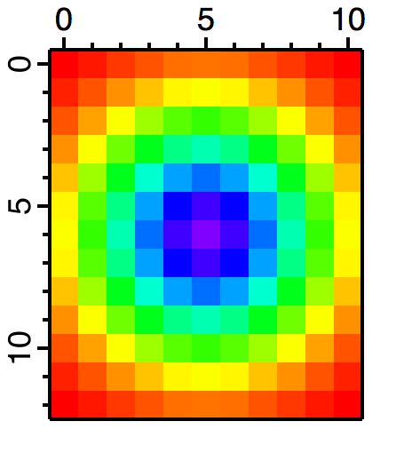
Figure 1: Low resolution pixelated image of p10.

INTERPOLATION EXAMPLES FOR GRIDDED DATA

If you want to get a single interpolated value for an arbitrary XYZ point inside the volume defined by ddd, e.g., (x=1.1, y=2.25, z=3.7) you can use:

If you need to interpolate a whole set of points that are not sampled on a rectangular grid, load their XYZ positions on a triplet wave and use Interp3DPath.  For example, we create a path containing 4 XYZ triplets:

Perform the interpolation:

If you need to interpolate the data to a new 3D wave of dimensions (100,150,200):

Create the wave:

Set the wave scaling to match the range of the original 3D wave:

and finally compute the interpolated values:

To find the interpolated plane corresponding to ddd[][][10] we first compute the new index using:

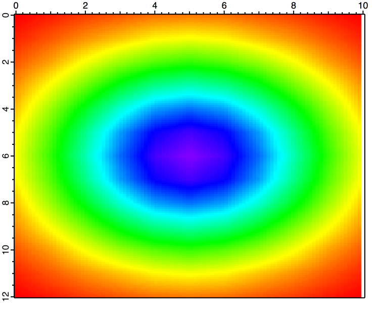
Figure 2: Image of layer 142 of new3DWave which is the interpolated form of layer 10 of the original data.

Note that the last row of p10Interp contains NaN values (shown in white above).  Normally interpolation routines return a NaN when the interpolation point is outside the domain of the data. In this case, the last row is 99 which corresponds to x value:

But x=10 should be part of the domain of the data, e.g.,

The reason for the NaN becomes apparent when executing instead

In other words, since Igor stores the wave scaling as two parameters, start and offset, copying the scales adjusts the start and offset but they are subject to floating point roundoff with the result that row 99 of new3DWave corresponds to x that is slightly larger to be out of bounds for the interpolation.

A pragmatic solution to this problem is to reduce the size of the offset parameter, e.g.,

Re-executing the interpolation:

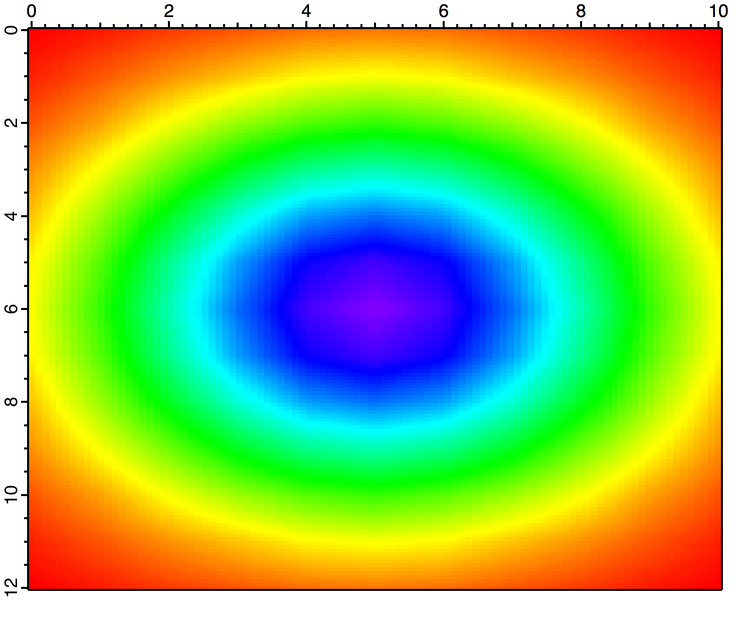
Figure 3: Corrected interpolation to avoid some NaNs on the boundary.

3D SCATTER DATA INTERPOLATION

Scatter data in this context takes the form of a 4-column wave where the first three columns contain the XYZ positions where the data were sampled and the last column contains the scalar values associated with each position.

The interpolation of 3D scatter data provides a continuous scalar value for any point inside the convex domain defined by the set of XYZ locations.  Igor returns NaN for points outside the convex domain.

In the following example I create a random sample of 500 points from the same data set we used above:

Next I compute the 3D triangulation of the data.  In this case the volume is subdivided into tetrahedra (not triangles).

The default result of Triangulate3D is stored in the wave M_3dVertexList.

If you want to interpolate only the plane corresponding to z=10 you can execute:

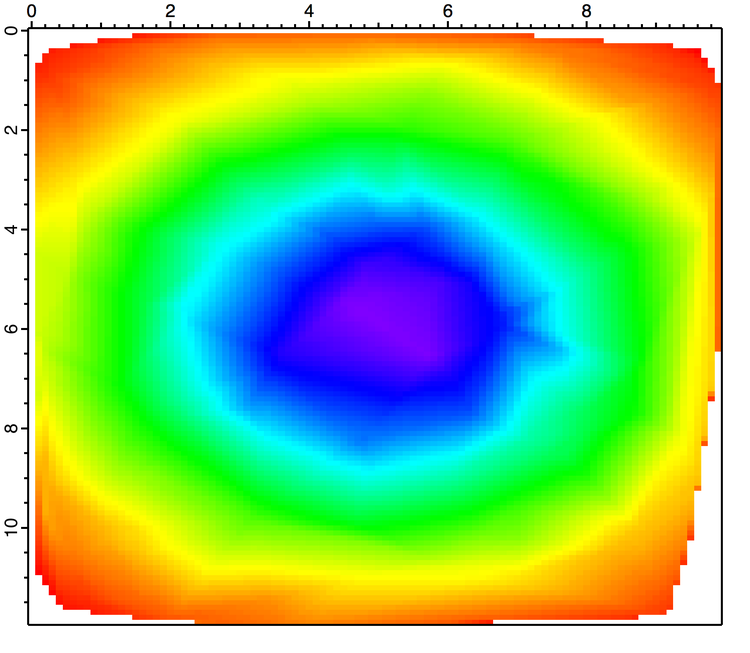
Figure 4: 3D interpolation of scatter data.

Note that you have NaNs in the corners suggesting that the random sampling of 500 points did not include edge points in this plane.  The interpolation, as in the 2D case, works by identifying the tetrahedron in which the interpolated point falls and then computing the interpolated value using the barycentric coordinates.

If you are interested in examining the details of the calculation you can execute instead:

and then display the tetrahedra in Gizmo using a regular path object.

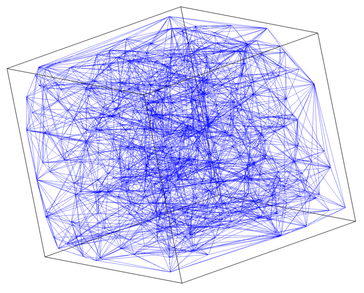
Figure 5: The tetrahedral decomposition of scatter data.  Here the density of points (500) makes it difficult to observe interior details but the absence of data from the corners is evident.