Triangulation and Interpolation on the Surface of a Sphere

This post is the third part of a multiple part series covering triangulation and interpolation using Igor Pro 7.

• Part 1: Planar Triangulations
• Part 2: Degeneracy and Sampling on a Rectangular Grid
• Part 3: Triangulation on the Surface of a Sphere and Triangulations in 3D
• Part 4: 3D Interpolation

In the previous two posts of these series I looked at triangulation and interpolation in the plane.  In this post I consider triangulation and interpolation when the data are sampled on the surface of a sphere.  Without loss of generality, we may consider a set of points {x, y, z} such that x^2+y^2+z^2=1.  

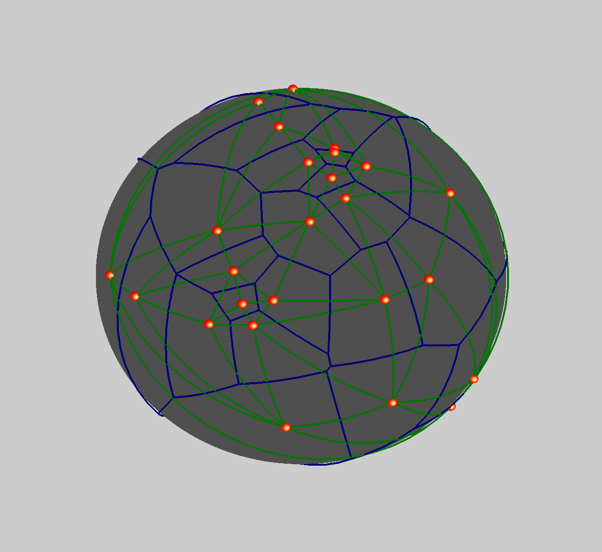
Figure 1 shows 25 random points on the surface of a sphere together with the Delaunay triangulation and the corresponding Voronoi tessellation.

Figure 1: 25 random points on the surface of a sphere.  Delaunay triangulation shows in green and Voronoi polygons are in blue.

The random set was generated using the function:

You can perform the triangulation on the surface of the sphere using the command:

The operation creates the wave M_TriangulationData that contains all the relevant information for drawing Figure 1.  In most situations you would not be interested in the triangulation details. Instead, you would use the wave M_TriangulationData to interpolate scalar data on the surface of the sphere given scalar values sampled at the regionalScatter locations say {vi}.  To compute the interpolated data you need three waves:  the first wave is M_TriangulationData that you got from SphericalTriangulate.  The second wave (dataPointsWave) is a 4 column wave that combines the scatter XYZ locations (regionalScatter wave) in the first 3 columns and {vi} as the 4th column.  You can create this wave using the command:

The third wave is a triplet wave that specifies the XYZ target locations on the sphere where you want to compute the interpolated values.  There are really no restrictions on the target locations wave as long as the XYZ triplets lie on the surface of the sphere.  If your target is a flattened image, e.g., some projection of the sphere, you can use the required XY resolution of the image and the projection mapping to create a target triplet wave of points on the surface of the sphere.

If you are using Gizmo to display the result of the interpolation, practical consideration suggest that the target wave should match the XYZ points of a parametric surface representing the sphere.  Note that in general you can convert a parametric wave into a triplet wave using:

You can perform the spherical interpolation using the command: 

The result is stored in the wave W_SphericalInterpolation and contains sequential scalar values corresponding to rows in paramTripletWave.  One way to display the interpolated values is to create a color wave for the parametric surface representing the sphere.  This is accomplished using the function:

The following example of interpolation on the surface of a sphere uses the procedure described above to analyze EEG data.  In this application EEG signals are measured by a standard net of sensors placed on a human head which, for the purpose of the analysis, is approximated by a spherical shape.  The known locations of the sensors replace the regionalScatter data in the example above.  The EEG signals are measured simultaneously at all sensors and their values at some time t0 correspond to the scalar set {vi} above.  The result of the interpolation is shown in Figure 2 which consists of three Gizmo subwindows displaying the same data at different orientations.

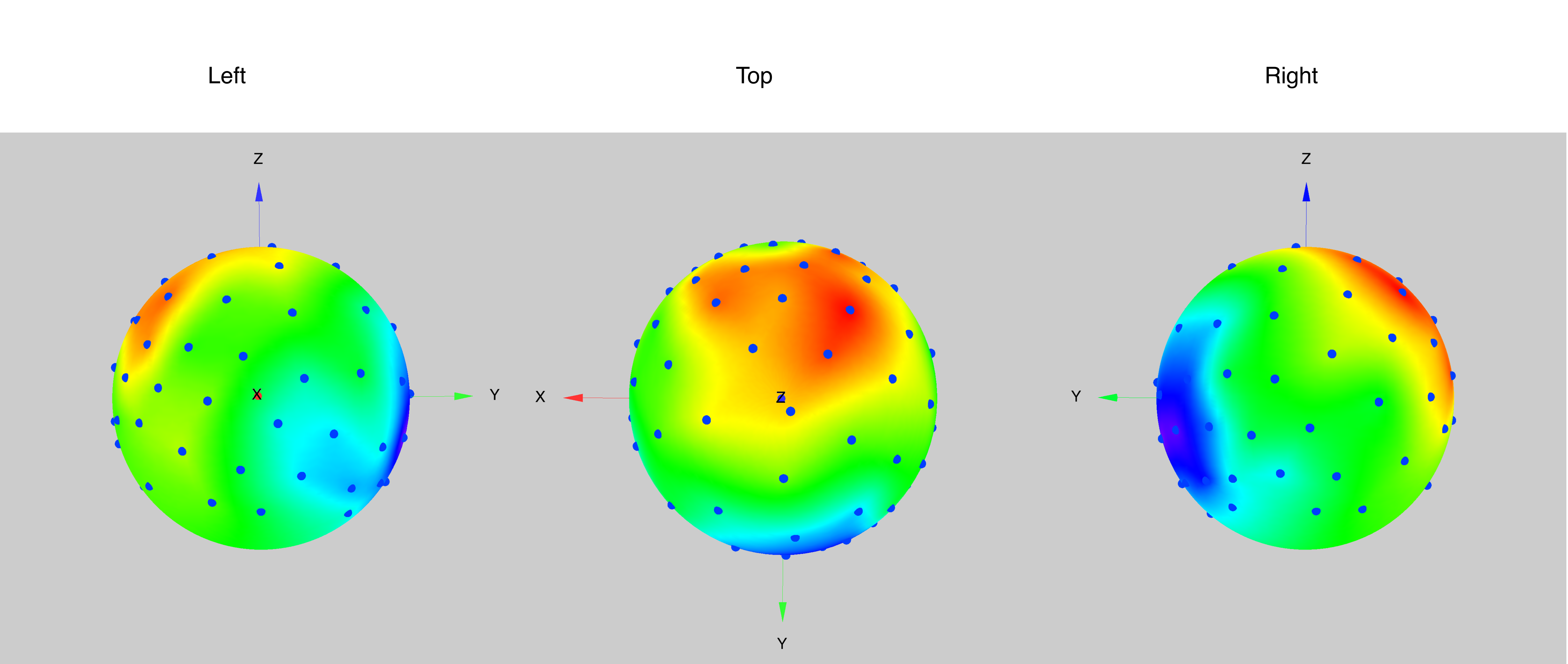
Figure 2: Three views of interpolated EEG signals

For more information about the EEG signal analysis see: 
http://www.gc.cuny.edu/Page-Elements/Academics-Research-Centers-Initiatives/Doctoral-Programs/Speech-Language-Hearing-Sciences/Research-Labs/Developmental-Neurolinguistics-Laboratory/Research-Highlights.