Baseline Fitting

Baselines is a baseline fitting utility for spectroscopic data.
How to use the Baseline Fitting package
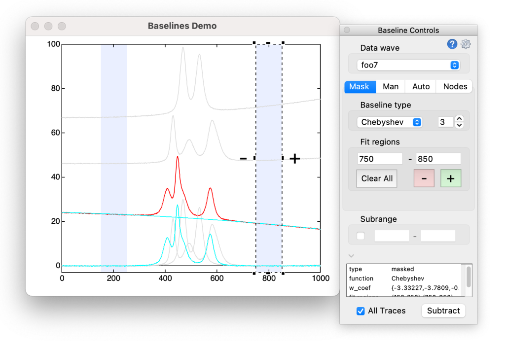
To get started, plot all of the waves that need baseline correction in a graph window. The waves may be vertically offset as you please. Select 'Baselines' from the analysis menu to attach the 'Baseline Controls' panel to the top graph. Traces in the graph will be recolored (unless the trace recoloring option is turned off in the settings panel) so that the selected trace, together with a preview of the baseline and baseline-subtracted waves, are the only non-grey traces. Traces are reset to their original colors when the 'Baseline Controls' panel is closed. Select a spectrum and baseline type from the popup menus in the control panel. The four tabs select between four 'families' of baseline algorithms: masked function fitting, manual function fitting, automatic baselines that process the input data to estimate a baseline, and 'node' baselines (splines and Chebyshev polynomials) that are interpolated between node positions selected by the user. Baselines works with both waveform and x-y traces, but not with 2D waves. Clicking on the cog icon opens a control panel where you can adjust the settings for baseline fitting. Close the main 'Baseline Controls' panel to clean up after fitting. Note that baselines uses cursors C through J, so don't try to use them for other purposes in the baseline fitting graph window.
Baseline Functions
Most of Igor Pro's built-in curve fitting functions can be selected as a baseline fit function. The fit coefficients are stored in the wave W_Coef, in case you need them for further processing. Some additional functions are selectable in the masked- and automatic-fitting tabs. These are described in the following sections.
Some baseline functions have a 'peak' option. When the 'Peak' checkbox is checked, the first coefficient of the fit function is set to the baseline reference value, meaning that these are peak functions with no vertical offset. The fit coefficients are described in the help for built-in curve fitting functions.
The Planck function uses Planck's law to fit a black-body radiation spectrum. Select the x-units of your data from nm, μm, wavenumbers, and Å. The temperature (in kelvin) that best fits the data is stored in W_Coef[0] and in the wavenotes of output waves.
The Chebyshev and Chebyshev2 baselines fit a Chebyshev series of the first and second kind, respectively. The setvariable control sets the maximum Chebyshev polynomial order, with an upper limit of 30, i.e. 31 fit coefficients. The arguments for the Chebyshev polynomials are shifted from the x-range of the data wave to the [-1, 1] interval. The coefficients of the best-fit Chebyshev series are saved in the wave W_Coef. Note: fitting a high-order Chebyshev series to a large number of points may be rather slow.
The tangent baseline (mask tab) will attempt to find a horizontal tangent if one fit region is selected, and a common tangent if two regions are selected. Each region is fitted with a cubic function, so the fit will be successful only if the selected regions can each be fit nicely with a cubic function, and if a horizontal or common tangent can be found with contact points within the selected regions. The coefficients for the tangent line are stored in W_Coef and are written to the wavenotes of output waves, together with the coordinates of the tangent points.
It is also possible to define your own baseline type. Custom baseline functions can be selected in the baseline type popups in the masked-region and auto tabs. See user-defined baseline functions for an explanation of how to add your own baseline types.
Some other baseline types that are specific to automatic fitting are described in the Auto Fitting section below.
Masked Fitting
Use the graph marquee tool (click and drag) to select a region of the spectrum, then use the + and - buttons (buttons adjacent to the marquee or the ones in the control panel) to add or remove a fitting region. Alternatively, keyboard shortcuts can be used in place of the buttons for adding and removing fit regions; the default keys are + and -, respectively. The baseline is determined by a leastsquares fit of the chosen function to data that fall within the selected regions.
Manual Fitting
The manual baselines allow you to create a baseline by positioning the cursors. The constant, line, and poly functions create a baseline that passes though all of the cursor positions. For Gaussian and Lorentzian functions, one cursor sets the baseline y-offset, the other sets the peak position and height, and the horizontal distance separating the cursors sets the peak width parameter. For sinusoidal baselines, the amplitude is set by the vertical offset of the two cursors and the number of complete cycles that should appear between the cursors can be adjusted in the baseline control panel.
Auto Fitting
The arc hull type baseline adds to the spectrum a circular arc with adjustable depth (i.e., the spectrum is bent), and the lower portion of a convex hull is calculated for the resultant spectrum. The baseline consists of the sum of the arc and the convex hull. Adjust arc depth using the SetVariable control to find an optimal value. Arc depth increments by 10% of its value and has y-axis units. Setting arc depth to zero creates a convex hull (a.k.a. 'rubber band') type baseline. For X-Y data, the X wave needs to be monatonic for arc hull calculation. Note that baseline segments can be convex or concave depending on the sign of the depth variable. The arc hull algorithm is not iterative.
Hull Spline: baseline is a cubic spline using the convex hull as nodes. When arc depth is non-zero the nodes are more like a subset of alphashape vertices. Adjust Smooth and Depth parameters to produce an optimal number of nodes. The hull spline algorithm is not iterative.
All other functions are fitted iteratively. Any fit point with a negative residual (positive if the negative peaks checkbox is selected) is replaced by the corresponding point from the input data after each iteration, thus eliminating points with a positive residual, so ultimately eliminating peaks from the fit. The fit output is used as the input for the next iteration. The algorithm is similar to that described by Lieber and Mahadevan-Jansen (2003) Applied Spectroscopy 57: 1363-1367. For the first eight iterations only points with a residual above 50% of the greatest residual are eliminated.
The spline function fits a smoothing spline. Adjust the estimate of noise level to optimise the fit.
Pre-smoothing: the baseline is calculated for a smoothed copy of the spectrum, then subtracted from the original. With the right choice of smoothing factor, the baseline will pass through spectroscopic noise rather than underlying the noise. Note that the baseline-subtracted output is not smoothed with respect to the original data, the smoothing is used only for calculating the baseline.
Negative Peaks: subtract the top part of the convex hull, or fit to the top of the spectrum. Useful for dealing with downward facing peaks, or for when you have a reverse-scaled vertical axis. The negative peaks setting is also adjustable in the settings panel, and affects the guesses for y positions of spline nodes.
Use Convex Hull at Start: In the first iteration, the baseline function is fit to the lower (upper for negative peaks) part of a convex hull of the input data. For some spectra this reduces the influence of peaks on the iterative baseline output.
Use the alt- (option- on the Mac) and shift-keys to respectively decrease or increase the increments when clicking the up and down buttons of the arc depth and sd noise estimate SetVariable controls.
Node Baselines
Node-type baselines are interpolated between node positions selected by the user. When 'edit mode' is active the nodes can be moved. The baseline updates as the nodes are repositioned. In edit mode you can add a new node at any position on the graph by positioning the mouse cursor and clicking while holding down the control key. Nodes may be deleted by clicking them with the alt/option key held down. Clicking the (moveable) button in the graph window or the 'edit mode' checkbox on the control panel will toggle between node editing mode and 'normal' mode where you can interact with the graph as usual. Cubic and smoothing splines are calculated using Igor's Interpolate2 operation. Cubic splines are calculated with 'natural' ends. Piecewise cubic Hermite interpolating polynomial (PCHIP) and Akima spline types can have tighter bends and less overshoot than a cubic spline. When a Chebyshev series of the first or second kind is selected, the maximum polynomial order, Nmax, is set using the setvariable control; when the number of nodes, n, is smaller than Nmax+1 the series will be truncated at order n-1. The coefficients of the Chebyshev series are saved in the wave W_Coef.
When a node type baseline is subtracted the node positions are saved in a 2D wave and can be later reloaded. Selecting a trace in the 'data wave' popup menu will reposition the nodes by adjusting their vertical positions. Clicking the node reset button resets horizontal and vertical node positions. The default algorithm guesses node positions by first fitting an auto-type baseline. Clicking the reset button with the shift key held down will position the nodes on the trace rather than guessing their positions. The horizontal positions are not changed unless there are insufficient nodes within the x-range of the new trace.
Subrange Fitting
Enable subrange fitting by clicking the checkbox and select a subrange by adjusting the values in the setvariable controls or by dragging the vertical cursors. When a baseline is subtracted, points within the selected range of any existing output wave are overwritten. For baselines in the mask, manual and spline families, this setting affects only the baseline subtraction process: the baseline calculation includes masked regions, cursors or nodes outside of the selected region. For algorithmic baselines (Auto tab), the data within the selected region are used to calculate the baseline, so adjusting the output range also changes the baseline. Spline nodes are not saved for subranges.
If a baseline has already been subtracted from the selected trace, points outside of the subrange will be filled with the existing values in both the baseline and baseline-subtracted output preview.
Show/Hide Baselines Info
Click on the info icon to display settings and fit coefficients for the selected baseline. Right-click in the information display area to copy the displayed information to the clipboard. Click the disclosure triangle to toggle the information display. The displayed information is a preview of some of the parameters that are stored in the wavenotes of output waves after baseline subtraction.
Subtracting Baselines
The 'Subtract' button will make copies of baseline and baseline-subtracted waves. These, together with any other output waves, can be saved in either the current data folder, or in the same location as the input data wave, or in a subfolder of either of these. If the 'Save Waves in Subfolders' option is checked in the settings panel, a subfolder with a name like 'baselines_auto_archull' will be created. The names of the output waves are formed from the input wavename, together with a suffix as defined in the settings panel. Use the subrange setting to subtract baselines in a piecemeal fashion.
If the "All Traces" checkbox is checked, the subtract button will fit and subtract a baseline, using the current settings, from each of the eligible traces in the plot. A baseline and baseline-subtracted wave is created for each trace. In this way, if you have found baseline settings that work well for a large set of data, baseline fitting can be done very efficiently. Spline fitting with All Traces checked guesses a y-position for the nodes for each trace.
Note that output waves with the baseline and subtracted-wave suffixes defined in the settings cannot be chosen as data waves for baseline fitting. If you want to subtract a sequence of baselines from one wave, edit the suffix in the settings panel after each baseline subtraction, or rename the output baseline-subtracted waves between fits.
Baseline fit parameters are saved in the wavenotes of output waves. When a baseline subrange is subtracted, the baseline parameters for the subrange are appended to the wavenotes of the output waves.
User-Defined Baseline Functions
You can define your own baseline type by creating two functions. The first is the fit function, which must have the FitFunc procedure subtype. Choosing 'new fit function' in Igor's curve fitting dialog will create a function with the correct format. The function should be saved in a procedure window of your choice.
A second function is required to set the initial guesses for the parameters used in your fit function. The name of the function is formed by appending "Guess" to the name of the fit function. The data-wave, x-wave and mask wave are passed to the guess function and can be used to choose optimal estimates for the fit parameters. The function must store the values of the initial guesses in a wave named "W_coef" in the current data folder.
Here is an example:
Function MyBaseline(cw, x) : FitFunc
    Wave cw // the coefficient wave
    Variable x // the independent variable

    // edit this part:
    return cw[0] + cw[1] * x
End

Function MyBaselineGuess(yw, xw, mask)
    Wave/Z yw, xw, mask
    // mask wave reference will be null if fit type is not masked
    // xw wave reference will be valid only if w_data is plotted vs xw
    // the waves passed to this function may represent a subset of the full
    // input data if subrange fitting is active

    // edit this part to store the initial guesses in the wave w_coef:
    Make/D/N=0/O W_coef
    W_coef[0] = {1,1}
End
If the code above is copied into the ProcedureWindow and compiled, the 'MyBaseline' baseline type will be added to the choices for auto and mask fitting. Acceptable names for fit functions are limited to 32 characters and must not be the same as a built-in fit type. Note that the waves xw and mask must be declared with the /Z flag. You can also provide an all-at-once style fit function. The fit function is used both for fitting and to calculate values for the baseline wave. To make your all-at-once function work for both waveform and x-y traces the function must check for the existence of the x-wave:
Function AllAtOnceBaseline(Wave cw, Wave yw, Wave/Z xw) : FitFunc

	if (!WaveExists(xw))
		Duplicate/free yw, xw
		xw = x
	endif

	// edit this part:
	yw = cw[0] + cw[1] * xw

	return 0
End

Function AllAtOnceBaselineGuess(Wave yw, Wave/Z xw, Wave/Z mask)
	// edit to store the initial guesses in the wave w_coef:
	Make/D/N=0/O W_coef
	W_coef[0] = {1,1}
End
When your all-at-once fit function is called for fitting, Igor's FitFunc operation will supply an x-wave, regardless of how the data are plotted. For assigning values in the baseline wave, the xw wave reference will be null for waveform data. Guess functions have the same format for both type of fit function.
Installing this package
- Consider using the IgorExchange Installer to install Baselines.ipf in the User Procedures folder.
- The Procedure Loader can be used to load or unload files stored in the User Procedures folder.
Project Details
Current Project Release
Baselines IGOR.7.00.x-5.14
| Release File: | Baselines514.zip (107.92 KB) |
| Version: | IGOR.7.00.x-5.14 |
| Version Date: | |
| Version Major: | 5 |
| Version Patch Level: | 14 |
| OS Compatibility: | Windows Mac-Intel |
| Release Notes: |
adds saving and loading of masked fit regions |

Forum

Support

Gallery
Igor Pro 10
Learn More
Igor XOP Toolkit
Learn More
Igor NIDAQ Tools MX
Learn More
If anyone is watching this space and would like to test a pre-release version of this project, let me know. It's a major rewrite, and there will likely be bugs. Once the worst of the bugs are shaken out I will release as version 4.
May 28, 2021 at 01:32 am - Permalink
This is a pre-release beta for version 4.
Edit: version 4 is released.
June 12, 2021 at 03:18 am - Permalink
This is a terrific contribution, Tony!
I just recommended it to a customer needing bulk baseline removal using the mask feature.
September 20, 2021 at 02:00 pm - Permalink
Thanks, Jim.
I'm glad to hear that others are finding it useful. I'm always curious to find out what kind of spectroscopic data other people use this project for. My colleagues and I use it mainly for baseline-correcting infrared and Raman spectra.
September 24, 2021 at 05:41 am - Permalink
Hi Tony,
Absolutely fabulous and really timely since I am reviewing some fitting algorithms for XRD data.
Question: If I wanted to start with a simple hull arc baseline using the default settings, what would the procedure be to be able to call it from a function? I would like to set up on some representative samples and then batch process a large number of spectra.
Andy
April 27, 2022 at 03:45 pm - Permalink
Hi Andy,
I'm glad that you like it!
All of the code is based around the GUI, so if you want to call a function without running the GUI I don't think that will work. Almost all functions take a structure as a parameter, so you'd have to do some tinkering if you want to call functions from your own code.
Or perhaps you want to invoke the GUI from your own function? That is as simple as building a graph and calling baselines#initialise(). You could simulate some GUI actions by loading the structure for a control and passing it to the control procedure, or there may be some other way to do it. Some more details about what you have in mind would be helpful.
April 28, 2022 at 12:44 am - Permalink
Dear Tony,
We tried Baseline Fitting IGOR.6.30.x-3.13 on our Igor 6.37, but it failed to compile (see attached screenshot). Is there a version compatible with Igor 6.37? Thank you very much.
June 26, 2022 at 08:25 pm - Permalink
Version 3.13 was missing a line of code at the top of the file:
The omission was fixed in the next release, but I see that the next release ended support for Igor 6.x. Adding the #include line to baselines,ipf should fix that particular problem. Sorry for the inconvenience.
If you find that the baseline fitting user interface works well for your needs, I recommend an upgrade to Igor 9. There were some significant improvements for Baselines version 4.x. You can make a comparison by installing the demo version of the current Igor release and the most recent version of the Baseline Fitting package.
June 27, 2022 at 12:08 am - Permalink
In reply to Version 3.13 was missing a… by tony
Thank you @Tony . Adding the code line solved our problem.
June 27, 2022 at 01:10 am - Permalink
Hi Tony, I updated to your new version 4.7 and (just our of interest) tired to open the help, but it does not work anymore for some reason. The Help Browser displays the topic titles but no window is opened when clicking on any of them or the help button in the panel. It was working fine in 4.62. Do you have any idea what is going on? I am on Windows 10 and Igor 8 / 9.
October 26, 2022 at 04:24 am - Permalink
That's strange. I just opened the help file that I uploaded with the release and on my mac it looks the same as my already compiled help file.
Maybe there are platform-specific issues that I haven't anticipated.
Here's the help files that shipped with versions 4.70 and 4.60. Do either of those work for you?
I've also added a file in which I replaced a potentially problematic character :)
October 26, 2022 at 06:27 am - Permalink
Hi Tony, I found out what is going on: The window position of the help seems to be saved into the .ihf file as well and it seems that from version 4.7 onward the window opens to the far right, outside of my visible screen area (on a 1080p display). If I retrieve the window I can see everything just fine. Here version 4.71 is better because it opens somewhat more to the left, inside the visible area of my screen. I guess you need to save the notebook when it is rather close to the top left, but I do not know how this works internally.
October 26, 2022 at 09:21 am - Permalink
I see, that's something I hadn't thought about adjusting before making a new release. I'll build a reminder into the 'prepare project release' code in the updater project so that I don't forget this for future releases. For anyone following this, look under Windows -> Control to find options to retrieve offscreen windows.
October 26, 2022 at 10:53 am - Permalink
Excellent package!!! Thank you.
I have one feature request -- I would like to have the option to store the results in a sub-folder in the working data folder. I would like to be able to specify that sub-folder name without having to click into the preferences wheel. The advantage is when I want to fit data sets with various types of baselines (e.g. linear versus spline). I would have the results immediately in different folders, avoiding the "overwrite??" dialog and allowing me easier viewing in the data browser to select a set to display. For example, below are the raw, linear, and spline fit results across a set of five spectra. I'd like to have had the baseline fitting spectra parsed immediately into their own sub-folders (e.g. linear and spline).
I might recommend that the user-defined functions be put in a separate procedure file that is #included to the main package. This would allow you to #pragma hide the main procedure so that users could not inadvertently mess it up. The requisite user-defined functions could be defined with a prefix such as BaselineUDF_, allowing users to write more than one type of baseline (that you then find with a FunctionName("BaselineUDF_*" ... ) search).
Again ... Excellent package. You deserve an applause and a round of your favorite beverage for making my yesterday evening an joyful one as I struggled with how to make IR spectra from five different samples that had gone through the same treatment really show that they were essentially having the same end chemistry despite the background changes.
November 18, 2022 at 09:48 am - Permalink
Thanks for the comments!
I think your feature request should be quite straightforward to work in. In the meantime, the Batch Renamer project may help to create some semblance of order. Another option is to drag the raw spectra into the different folders and use the same-as-source output folder option to make sure the output ends up where you want it. But subfolders are definitely doable.
November 18, 2022 at 11:34 am - Permalink
Tony- I just had a question from a customer who wants to remove a baseline but avoid any negative values. Is there a way to do that? I saw that she had found this package, so one hurdle jumped already.
November 18, 2022 at 02:56 pm - Permalink
I think that needs to be a bit more specific - do you mean that the output (data minus baseline) has to be non-negative? A convex hull?
November 18, 2022 at 03:15 pm - Permalink
An 'arc-hull' baseline with no pre-smoothing gives output >= 0.
November 18, 2022 at 03:22 pm - Permalink
Dear Tony,
I must say this Baseline package is just outstanding.
I am using it from last couple of versions now for bulk baseline subtraction of my Raman and IR data. It really reduces a considerable burden of data pre-processing.
However, I want to put a small request. If it can be managed somehow, it will be great.
The mostly use Auto Fitting for bulk data and I just manually adjust the nodes for each individuals before doing Subtract,
Now as the Data Wave lists the waves from the graph in the same order as they appear in the graph, if I chose the top most wave from the list, the top wave is actually at the back of all waves in the graph. As all of my data are very close by, I is very difficult to adjust the nodes. As a remedy, what I am currently doing is, manually choosing the last wave in the Data Wave list everytime I am doing the processing.
It would be nice if the waves is sorted in the list as from front to back order (opposite to trace order in the graph).
The trace order of W_base, W_nodes, W_sub are fine. I have attached a screenshot of my data for you reference.
Thank you once again for providing us such an fantastic package.
With regards,
Saha
March 17, 2024 at 10:52 pm - Permalink
Thanks, Saha, for the kind words.
I think I see your workflow - you're using the option to remove the original trace after baseline subtraction, and you want the selection to jump to the frontmost trace. It's an easy fix. I'll put out a new release that works that way.
March 18, 2024 at 04:27 am - Permalink