Spectra Wave Arithmetic - Match 1D/2D waves to calculate differences, sums etc.

This package provides a user interface and programming environment for aligning and comparing two 1D / 2D waves and calculate for each overlapping point: output = f(modified input data, reference data). The input is modified using the UI controls and compared against a reference wave. Available Modes are:

• Subtraction (-)
• Addition (+)
• Multiplication (*)
• Division (/)
• Average
• Percent difference (the difference normalized by the average in %, i.e., (A-B)/(A+B) * 200)
• A custom user equation

The input wave can be shifted, offset and scaled. The original purpose was to calculate differences, hence the name Difference Generator. Latre versions added support for addition, multiplication, division, percent difference and arbitrary equations. 

The source waves of both the data to be modified and the reference is never altered. The calculation is done on temporary data, and any modification (named with ending "_mod") and the result of the arithmetic operation are exported as separate output waves. The default ending for naming the output is "_dif" for subtraction, "_sum" for addition, "_mul" for multiplication, "_div" for division, "_pdif" for % difference and "_calc" for custom formulas. Settings are saved within the output wave's notes and will be reloaded automatically upon resuming with the same input. The UI is folder aware. 

I tried my best to test everything thoroughly, but you should verify the correct behavior yourself to be sure. Bug reports and suggestions for new features are always welcome.

Graphical User Interface (UI) controls - 1D data

Select one or two waves in the Data Browser and then navigate to 'Spectra Tools' → 'Compare and Modify Data....' in the main menu or use the command line:

WaveArithmeticUI(WaveToEdit)

or alternatively:

WaveArithmeticUI(WaveToEdit,refwave=ReferenceWave)

The second wave selected in the Data Browser or provided via the optional 'refwave' parameter is pre-selected as reference. This is an overview of the controls (here, for modifying 1D data):

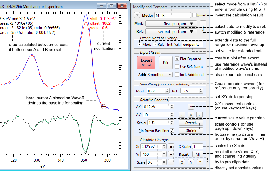
The modified wave and the reference wave can be selected via the drop-down menu and their role switched via the ] button. If Extend Data to Overlap is active the source or reference data is extended by either repeating the data's endpoints or by inserting the specified value set via Init. Val.. The reference data is extended to the range of the modified data and vice versa (there is no effect if the data overlaps already fully). This is most useful when the data already has flattened out close to a baseline or even zero  at the edges, so that the error of this artificial extension is small.

Operation Mode:

• Choose a preset from the (▼) drop-down menu: M - R subtraction (- key), M + R addition (+ key), M * R multiplication (* key) or M / R division (/ key), (M + R) / 2 average or (M - R) / (M + R) * 200 percent difference.
• Any custom equation may be entered directly using M (modified input data) and R (reference data).
• The result can be inverted (flipped along the Y or Z axis) with the Invert checkbox (i key).

When you are done:

• Export & Exit will export the result and modification as separate waves and then closes the UI.
  The exported waves are plotted in a graph when the Plot Exported checkbox is active. All previous graphs with the same data are updated as well to reflect the new settings. All settings are saved with the output and will be reapplied upon reloading. See further below for an explanation how the data is saved including the purpose of the 'Use Ref. Name' setting.
• Exit will close the UI without saving anything.
• Use the Add drop-down menu to select the type of post-processing: smoothing, integration or derivation of the result. Activating the Incl. Additional item will export this post-processed data as well (name ending '_smt', '_int' or '_der').

Applying Changes to the Input Data:

• Shift in X / horizontal and Y / vertical directions using the arrow buttons (cursor keys on the keyboard).
• Scale using the stretch (page up key) and shrink (page down key) controls.
• The delta step of each modification can be set using the controls to the left.
• Absolute Changes in the lower section of the UI can be used to dial in the desired values directly.
• Pressing the = (equal) button next to each axis value will automatically pre-align or scale the data to match the reference in the respective direction. Hold Option (Mac) / Alt (Win) while pressing ‘=’ next to Scale to scale the data by using the total area instead of the minimum / maximum intensities.
• Use the Reset buttons for All modifications or individual changes of the X / Y shift or (*) scaling to undo modifications.

Smoothing:

• Both waves can be Gaussian broadened by setting the respective control. Smoothing of the reference data is only temporary and not applied to the input reference data. This setting is saved with the output and will be reapplied upon reloading. Use the home / end keyboard shortcuts to increase / decrease the smoothing value. Holding alt/option will change the value for the reference data. In case of 2D data, hold cmd/ctrl to change the Y smoothing value.

Further keyboard shortcuts: 

• Hold Cmd (Mac) / Ctrl (Win) for changes in steps of 0.5 times the current delta value.
• Hold Shift for changes in steps of 10 times the current delta value.
• Hold both Shift + Cmd / Ctrl for changes in steps of 0.1 times the current delta value.
• r key to ‘Reset All'
• p key to toggle ‘Pin Background’
• Hold Cmd (Mac)/ Ctrl (Win) while pressing ‘Reset All’ and the reference wave will be set to none.
• Hold Cmd (Mac)/ Ctrl (Win) while pressing ‘Export & Exit’ to export without closing the UI. This is useful to process many waves in quick succession by selecting the next one from the drop-down menu.
• Hold Option (Mac) / Alt (Win) while pressing ‘Export & Exit’ to force the 'Use Ref. Name' setting (this has the same effect as activating the check box).

Graphical UI controls - 2D data

2D data is loaded and processed in the same way. The data is now displayed as two overlapping images, with the reference data plotted as a semi-transparent layer on top of the input data. There are additional controls specific to 2D data (see below), such as additional controls to modify the third (Z) dimension:

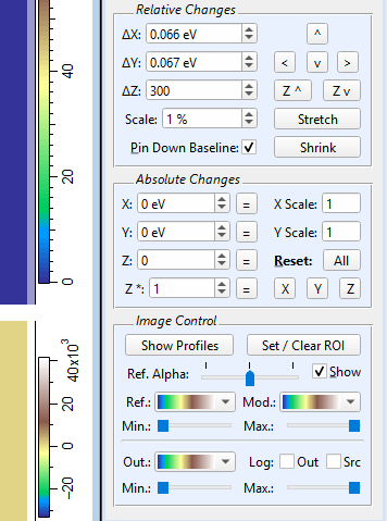
At the very bottom are additional controls to modify the image appearance:

• Ref. Alpha: The transparency (alpha value) of the reference data. Choose between fully transparent (slider to the left) and fully visible (slider to the right).
• Show (reference): Toggles the visibility of the reference image. Uncheck to hide. Can also be toggled with the s key on the keyboard.
• Image color and Range controls: Choose the color mapping for each image and adjust the displayed z-range via sliders.
• Log (colors): Switch to log color display for the output (Out) or source input data (Src).

Showing Profiles and Setting Region-Of-Interest (ROI):

To aid with alignment, the intensity profiles (i.e., sum) in X / Y directions can be displayed via the Show Profiles button. A side-panel will appear with two graphs, one for X and one for Y. Profiles will update automatically, you can immediately see the effect of each modification.

To limit the range from which the profiles and displayed min. / max. values are calculate, drag a marquee across the image over the region of interest you want to work with. Then, use the Set / Clear ROI button. Pressing the button again without a marquee on the graph will clear the ROI. You can alternatively use the right-click menu after dragging a marquee to set / clear the ROI. Limiting the range makes it easier to align / match a specific sub-region of the data.

How the result is saved

The result is exported to the folder of the input as 'wavename' +  "_mod"' for the modified data and  'wavename' +  mode-specific extension for the result of the calculation. The mode-specific extensions are:

• "_dif"' (subtraction)
• "_sum" (addition)
• "_mul" (multiplication)
• "_div" (division)
• "_avg" (average)
• "_pdif" (percent difference)
• "_calc" (custom formula)

All settings are saved inside the wave note of both of these output waves. Below is an example output, where 'first spectrum' was modified and 'second spectrum' was the reference:

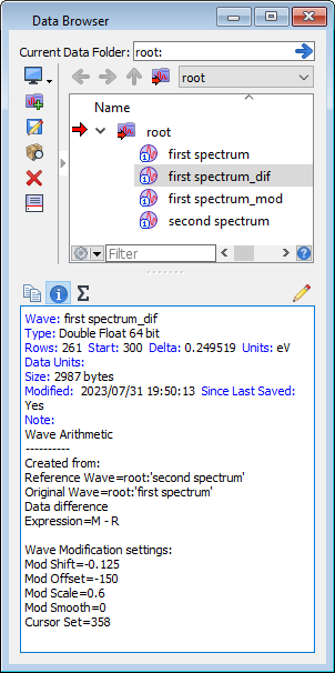
Loading the UI with the same initial data ('first spectrum' in this case) will reload the last session from the '_mod' (or '_dif' wave, if '_mod' does not exist). Note that loading a '_dif' or '_mod' wave directly will just start a new session (this makes it possible to create differences of differences etc.). The input and reference data can be in different folders, but the '_mod' or '_dif' wave should stay with the respective input in the same folder.

If neither a 'dif' (or 'sum', 'mul', 'div') or 'mod' wave with the same name is found in the input wave's folder, then the default settings are loaded. It is thus recommended to keep the result and modified waves together with the input in the same folder to be able to reload the settings later. What will be reloaded if you have mixed result waves from different modes? The loading hierarchy is 'mod' > 'dif' > 'sum' > 'mul' > 'div' > 'pdif'. For example, without the '_mod' and '_dif' waves present in the folder will load the settings from the '_sum' wave if present.

What is the purpose of the 'Use Ref. Name' setting?

Imagine the following scenario: You have measured 'baseline' data and then several data sets in succession like this:

1. baseline
2. measurement1
3. measurement2
4. measurement3
5. ...

Let's assume you want to remove the baseline from all measurements but each measurement data itself should not be altered (e.g., to preserve their relative shift or intensity). You instead can modify (shift, scale etc.) the baseline while comparing to each measurement and then save the result next to each data set using the Use Ref. Name setting.

Load the baseline as Modify and one measurement as Reference, then apply modifications as necessary (to the baseline). Since the role of the modified and reference data is reversed, this usually means you need to activate 'Invert'. Before exporting, activate 'Use Ref. Name' to save the result next to each measurement set. This will create a unique output for each measurement:

1. baseline
2. baseline_mod
3. measurement1
4. measurement1_dif
5. measurement2
6. measurement2_dif
7. measurement3
8. measurement3_dif
9. ...

What if you reload measurement1 but have conflicting settings in waves measurement1_mod and measurement1_dif? In this case, measurement1_mod is loaded according to the hierarchy 'mod' > 'dif' > 'sum' > 'mul' > 'div' > 'avg' > 'pdif'.

Running your own code:

You can generate outputs from two waves using the function: 

doWaveArithmetic(WaveArithmeticStruct s)

The WaveArithmeticStruct structure looks like this:

Structure WaveArithmeticStruct
	variable mode		// 1: Subtr. (M-R) 2: Add (M+R) 3: Multiply (M*R) 4: Divide (M/R) 5: Avg 6: %Diff => (default 1)
	char formula[100]	// free-form arithmetic expression: M & R as stand-in for orgWave & refWave; use instead of mode
	WAVE orgWave		// [mandatory] source wave to be modified - will NOT be modified in any way
	WAVE refWave		// [optional]  reference wave to compare  - will NOT be modified in any way
	WAVE cmpWave		// [optional] result of comparison between orgWave and refWave will be written here
	WAVE modWave		// [optional] modified wave - saves the scaled and shifted version of orgWave
	WAVE modRefWave		// [optional] modified reference wave - saves the smoothed version of refWave (if refSmooth > 0)
	WAVE srcConvKernel  // [optional] data to convolve with the input, e.g., for smearing.
	WAVE refConvKernel  // [optional] data to convolve with the reference.
    
	// all below parameters are optional
	variable/C orgSmooth	// Gauss width for smoothing / wave 1 (complex for 2D)	(default 0)
	variable/C refSmooth	// Gauss width for smoothing / wave 2 (complex for 2D)	(default 0)
	variable refExtend	// extends the ref. wave to the full source range	(default 0)
	variable srcExtend	// extends the src. wave to the full source range	(default 0)
	variable extFillVal	// optional value to fill the extended region with	(default NaN)
	variable baselineXval	// x position of baseline				(default NaN)
	variable baselineYval	// y value (1D) or position (2D)of baseline		(default 0)
	variable baselineZval	// for 2D: z value of baseline				(default 0)
	variable baselineFixed	// baseline is omitted from Y scaling if set to 1	(default 0)
	variable invert		// invert the output in Y				(default 0)
	variable xShift		// modify wave 1: x displacement (in wave's units)	(default 0)
	variable yShift		// modify wave 1: y displacement (in wave's units)	(default 0)
	variable valShift	// modify wave 1: intensity displacement (offset)	(default 0)		
	variable xScale		// modify wave 1: x scale				(default 1)
	variable yScale		// modify wave 1: y scale				(default 1)
	variable valScale	// modify wave 1: y / z scaling				(default 1)
	variable UIpinToggle	// options related to user interface; don't use		(default 0)
	variable UIoptions	// bit options related to user interface; don't use	(default 0)
EndStructure

In your code, use the structure to pass the input waves and desired parameters to the function. You need to pass at least the input  data (orgWave). A modified version of this wave will be generated (the input will not be altered). If you want to specify where this modified data ends up, optionally pass modWave pointing to a target wave into the function. If you specify a wave for comparison (refWave) the arithmetic expression (default: subtraction) is evaluated between this reference and the modified input. The result is either written into an automatically generated output wave or into cmpWave if specified. A simple example could look like this:

Function CompareTest1D(WAVE in1, WAVE in2)

    STRUCT WaveArithmeticStruct s
    WaveArithmeticInitialize(s) // initialize structure parameters with defaults
    WAVE s.orgWave = in1
    WAVE s.refWave = in2
    s.valScale =  0.5	// scale wave1 (optional; wave1 will not be altered)
    s.xshift   = -0.02	// shift wave1 (optional; wave1 will not be altered)
    Print WaveArithmeticErrorMsg(doWaveArithmetic(s))
End

WaveArithmeticErrorMsg() generates a human-readable error message in case there is a problem. If official name-end tags (e.g., "_dif") are used then the output is fully compatible with the UI, i.e., settings are parsed when using the UI with the generated waves.

To apply smoothing via Gaussian convolution you can use the parameters orgSmooth (for the input wave) and refSmooth (for the reference wave). Note that the Gaussian is defined as a peak function, i.e., exp(-x²/w²), and not as a normalized Gaussian distribution, i.e., exp(-½ x²/w²). If a normalized Gaussian distribution is required, then the width w can simply be multiplied by √2.   Also, the full width at half maximum is FWHM = 2√(ln(2)) * w ≈ 1.6651 * w. Simple smoothing can be achieved as follows:

Function ConvolveTest1D(WAVE in1D)

    STRUCT WaveArithmeticStruct s
    WaveArithmeticInitialize(s)
    WAVE s.orgWave = in1D
    s.orgSmooth = 1.2    // smooth with a Gauss peak of width 1.2
    Print WaveArithmeticErrorMsg(doWaveArithmetic(s))
End

In case of 2D data, smoothing can be independently controlled for the x and y directions. The approach is the same as above, but a complex number must be passed to the parameter. The real part controls the x and the imaginary part the y direction. If one of the numbers is zero, then the convolution is switched off for the respective direction. A simple test could look as follows:

Function ConvolveTest2D(WAVE in2D)

    STRUCT WaveArithmeticStruct s
    WaveArithmeticInitialize(s)
    WAVE s.orgWave = in2D
    s.orgSmooth = cmplx(1.5, 0.75)  // smooth with a Gauss peak of width xw = 1.5 and yw = 0.75
    Print WaveArithmeticErrorMsg(doWaveArithmetic(s))
End

It is possible to apply smoothing with a numerical kernel (wave) as input to srcConvKernel (for the input wave) or refConvKernel (for the reference wave). The kernel should be properly centered and area-normalized, although the program makes sure to properly center and normalize any input. It is best to make sure the kernel is zero at the edges, i.e., any data should fall off as close as possible to zero and should not be offset in y (unless that is the purpose of the kernel). The kernel should also have the same delta spacing as the input data, although this is automatically cared for in the program as well. This test produces the same result as above (assuming the input in1D is unscaled):

Function ConvolveTest1Dkernel(WAVE in1D)

    STRUCT WaveArithmeticStruct s
    WaveArithmeticInitialize(s)
    WAVE s.orgWave = in1D
    Make/FREE/N=(21) kernel = Gauss(x, 10, 1.2/sqrt(2))  // smooth with a Gauss kernel of width 1.2
    WAVE s.srcConvKernel = kernel
    Print WaveArithmeticErrorMsg(doWaveArithmetic(s))
End

For 2D data you can use a full 2D kernel as input. But note that this might be slow depending on the size of the input and the kernel. In the worst case this calculation may take several seconds to minutes. It is possible to pass a 1D kernel to just smooth the input in one axis direction. The direction of the kernel determines the direction of the smoothing: a single-row wave will lead to smoothing in x while a single-column kernel smoothes in y:

Function ConvolveTest2Dkernel(WAVE in2D)

    STRUCT WaveArithmeticStruct s
    WaveArithmeticInitialize(s)
    WAVE s.orgWave = in2D
    Make/FREE/N=(21) kernel = Gauss(x, 10, 0.75/sqrt(2))  // smooth with a Gauss kernel of width 0.75
    MatrixTranspose kernel  // convert into a column vector => y smoothing
    WAVE s.srcConvKernel = kernel
    Print WaveArithmeticErrorMsg(doWaveArithmetic(s))
End

Settings inside the procedure header

The header contains settings as static constants which are used by the UI, and can be edited here if needed (rather not mess with these settings unless really necessary). For example, the name-end tags ('_dif', '_mod' etc.) can be altered here, should there be a conflict with other names in your work-flow (in fact, Igor's own Differentiate function also uses '_dif'):

static StrConstant kModEnd	= "_mod"					// label for modified data
static StrConstant kAuxEnd	= "_smt;_int;_der;"				// label for additional data
static StrConstant kOutEnd	= "_calc;_dif;_sum;_mul;_div;_avg;_pdif;"	// label for output data
static StrConstant kModePresets = "M - R;M + R;M * R;M / R;(M+R)/2;(M-R)/(M+R) * 200;"	// presets for the modes